Simulate a resolving-power-dependent profile from a fine isotope pattern

Sums a Gaussian peak of the appropriate width for each isotopologue in an isotope_fine_pattern result, at a chosen resolving power. At low resolving power, isotopologues that are close in mass merge into one apparent peak; at high resolving power they separate – this is what an Orbitrap or FT-ICR spectrum of the same ion actually looks like. Because abundance is already expressed as percent of the base peak, overlapping isotopologues sum the way real overlapping peaks do, so the simulated apex can exceed any single isotopologue's own abundance.

Usage

isotope_profile(pattern, resolution = 120000, oversample = 12, pad_fwhm = 6)

Arguments

pattern

output of isotope_fine_pattern (or any tibble(mz, abundance)).

resolution

resolving power (R = m/z / FWHM) AT the m/z of this pattern. If your instrument's resolving power is quoted at a reference m/z (the usual Orbitrap convention, typically 200), convert it first, e.g. R_ref * sqrt(200 / mean(pattern$mz)).

oversample

grid points per FWHM.

pad_fwhm

how many FWHM of m/z padding to add on each side.

Value

A tibble with columns mz and intensity (percent of the base peak's abundance, same scale as isotope_fine_pattern()'s abundance column).

Author

Jan Stanstrup, stanstrup@gmail.com

Examples

# \donttest{
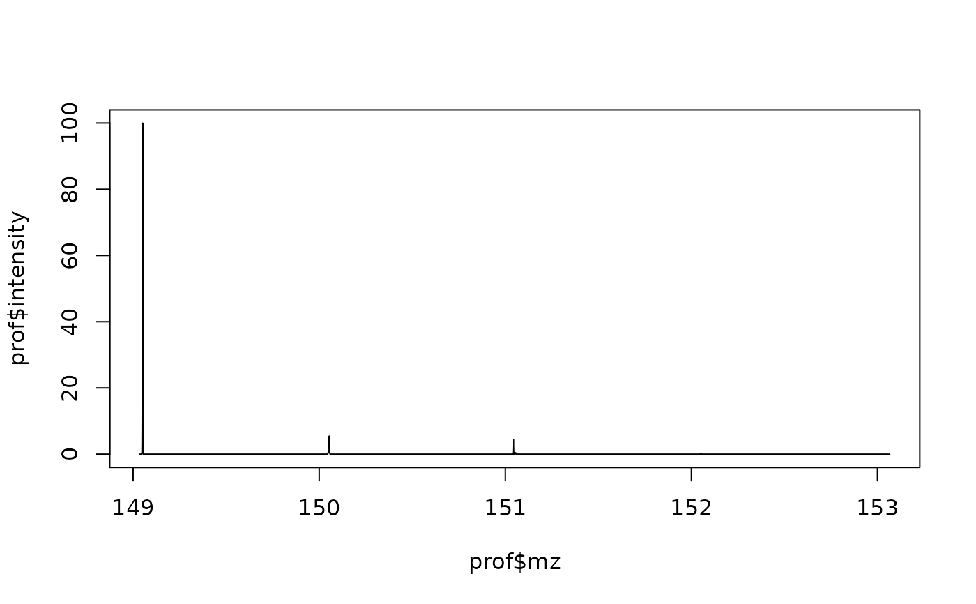
pat  <- isotope_fine_pattern("C5H11NO2S")
prof <- isotope_profile(pat, resolution = 60000)
plot(prof$mz, prof$intensity, type = "l")

# }