Isotope fine structure is what happens when a nominal M+1 or M+2 level contains several isotopologues at slightly different exact masses. At M+1, every peak comes from substituting exactly one atom with its heavy isotope — ¹³C, ²H, and ¹⁵N are the most prominent contributors (oxygen and sulfur are better known for M+2: ¹⁸O and ³⁴S are five times more abundant than ¹⁷O and ³³S). At M+2, single substitutions of two-neutron isotopes (³⁴S, ³⁷Cl, ¹⁸O…) appear alongside combinations of two M+1 isotopes. Whether your instrument resolves any of these as separate peaks depends on resolving power. This article explains the positions, walks through a concrete example, and builds the tools to simulate what a real spectrum would show.
M+1: one atom is a heavier isotope, but you get several exact masses
If you add a neutron to a nucleus, the mass increase is not exactly the free neutron mass (1.008665 Da). When the neutron binds, the nucleus releases some energy — and by E = mc², that released energy corresponds to a small mass deficit. The binding energy gain differs for every element, so each isotope has its own exact mass shift. All of the following contribute to the M+1 level, but they sit at genuinely different m/z values:
| ¹³C |
+1.003355 |
0 |
| ¹⁷O |
+1.004220 |
+0.9 |
| ²H |
+1.006277 |
+2.9 |
| ³³S |
+0.999388 |
−3.9 |
| ¹⁵N |
+0.997035 |
−6.3 |
The 9.2 mDa spread between ¹⁵N and ²H is larger than the mass accuracy of any modern high-resolution instrument. Whether your spectrum resolves them as separate peaks depends on resolving power and the compound’s elemental composition; the worked example below shows how to calculate that.
Why ¹³C tends to dominate M+1. The relative height of each peak is proportional to the isotope’s natural abundance multiplied by the number of atoms of that element in the molecule. ¹³C has 1.11% abundance per carbon, and organic molecules often contain many carbons — so the total ¹³C contribution (roughly n × 1.11%) quickly outweighs ²H (0.015% per H), ¹⁵N (0.37% per N), and the trace M+1 isotopes of O and S. A molecule with five carbons already has a ~5.5% chance of carrying one ¹³C, far above any single ¹⁵N or ²H contribution.
M+2: combinations and heavier isotopes
At M+2, two types of peak appear: two-neutron heavy isotopes (³⁴S, ³⁷Cl, ³⁸Ar…) and combinations of two M+1 isotopes. They sit at different exact masses:
| ¹³C + ¹³C |
+2.006710 |
0 |
| ¹⁸O |
+2.004220 |
−2.5 |
| ³⁷Cl |
+1.997051 |
−9.7 |
| ³⁴S |
+1.995796 |
−10.9 |
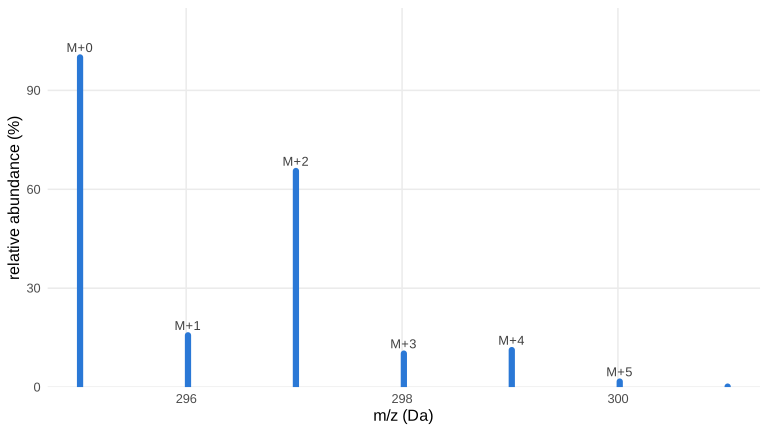
When a molecule carries several chlorines or one sulfur, these two-neutron isotopes can completely dominate the M+2 level. Diclofenac (C₁₄H₁₁Cl₂NO₂) is an extreme case: two chlorines at 24.2% each push M+2 to ~65% of M, an excess so large that no fine-structure measurement is needed to recognise it.
Show code
pat_dic  <- isotope_fine_pattern("C14H11Cl2NO2")
base_dic <- pat_dic %>% filter(label == "") %>% pull(mz)

coarse_dic <- pat_dic %>%
  mutate(nominal = round(mz - base_dic)) %>%
  group_by(nominal) %>%
  summarise(mz = base_dic + first(nominal), abundance = sum(abundance), .groups = "drop")

ggplot(coarse_dic, aes(mz, abundance)) +
  geom_segment(aes(xend = mz, y = 0, yend = abundance),
               colour = BLUE, linewidth = 2.2, lineend = "round") +
  geom_text(data = filter(coarse_dic, abundance > 1),
            aes(label = paste0("M+", nominal)),
            vjust = -0.6, size = 3.4, colour = "grey25") +
  scale_y_continuous(limits = c(0, NA), expand = expansion(mult = c(0, .15))) +
  labs(x = "m/z (Da)", y = "relative abundance (%)") +
  theme_minimal(base_size = 12) +
  theme(panel.grid.minor = element_blank())
Running example: methionine
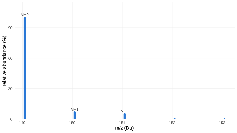
Methionine (C₅H₁₁NO₂S) is one of the twenty proteinogenic amino acids, present in every untargeted metabolomics run. It carries one sulfur, whose ³⁴S isotope sits at 4.25% natural abundance. Nothing about a coarse M+1/M+2 barcode makes that obvious: the bars look ordinary until you notice M+2 far exceeds what five carbons alone could explain.
Change formula here to run the same workflow for your own candidate:
Show code
formula <- "C5H11NO2S"   # methionine -- swap to your own candidate

pat     <- isotope_fine_pattern(formula)
base_mz <- pat %>% filter(label == "") %>% pull(mz)
coarse  <- pat %>%
  mutate(nominal = round(mz - base_mz)) %>%
  group_by(nominal) %>%
  summarise(mz = base_mz + first(nominal), abundance = sum(abundance), .groups = "drop")
Show code
ggplot(coarse, aes(mz, abundance)) +
  geom_segment(aes(xend = mz, y = 0, yend = abundance),
               colour = BLUE, linewidth = 2.2, lineend = "round") +
  geom_text(data = filter(coarse, abundance > 1),
            aes(label = paste0("M+", nominal)),
            vjust = -0.6, size = 3.4, colour = "grey25") +
  scale_y_continuous(limits = c(0, NA), expand = expansion(mult = c(0, .15))) +
  labs(x = "m/z (Da)", y = "relative abundance (%)") +
  theme_minimal(base_size = 12) +
  theme(panel.grid.minor = element_blank())
Five carbons predict M+2 from double-¹³C at choose(5,2) * 0.0107^2 * 100 ≈ 0.11%, roughly 40 times smaller than the 5.1% actually observed. Whenever M+2 badly overshoots what carbon alone predicts, suspect S, Cl, Br, Si, or a metal — the fine structure below names the specific isotopologue.
Step 1: build the fine-structure table
isotope_fine_pattern() reports each isotopologue separately, at its own exact mass, labelled by which isotopes produced it:
Show code
pat %>% arrange(mz) %>%
  mutate(mz = round(mz, 5), abundance = round(abundance, 4),
         label = ifelse(label == "", "M (monoisotopic)", label)) %>%
  knitr::kable(caption = paste("Every isotopologue of", formula, "above the default 0.01% threshold."))
Every isotopologue of C5H11NO2S above the default 0.01% threshold.
| 149.0511 |
100.0000 |
M (monoisotopic) |
| 150.0481 |
0.3653 |
15N |
| 150.0504 |
0.7896 |
33S |
| 150.0544 |
5.4079 |
13C |
| 150.0553 |
0.0762 |
17O |
| 150.0573 |
0.1265 |
2H |
| 151.0469 |
4.4742 |
34S |
| 151.0514 |
0.0198 |
13C, 15N |
| 151.0538 |
0.0427 |
13C, 33S |
| 151.0553 |
0.4110 |
18O |
| 151.0578 |
0.1170 |
13C, 13C |
| 152.0439 |
0.0163 |
15N, 34S |
| 152.0502 |
0.2420 |
13C, 34S |
| 152.0587 |
0.0222 |
13C, 18O |
| 153.0461 |
0.0105 |
36S |
| 153.0511 |
0.0184 |
18O, 34S |
Step 2: zoom into one nominal level
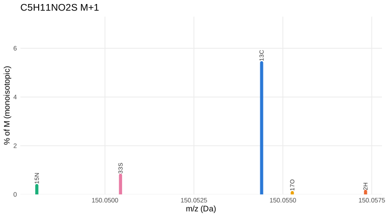
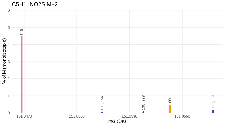
On the m/z axis, M+1 and M+2 each split into several distinct peaks:
Show code
plot_level <- function(pattern, level, title) {
  base <- pattern %>% filter(label == "") %>% pull(mz)
  d <- pattern %>%
    mutate(nominal = round(mz - base)) %>%
    filter(nominal == level) %>%
    mutate(element = sub(",.*", "", label),
           element = sub("^[0-9]+", "", element),
           col = ifelse(label == "" | grepl(",", label), "combo", element),
           col = ifelse(col %in% names(COL), col, "combo"))
  ggplot(d, aes(mz, abundance, colour = col)) +
    geom_segment(aes(xend = mz, y = 0, yend = abundance),
                 linewidth = 2.2, lineend = "round") +
    geom_text(data = slice_max(d, abundance, n = min(6, nrow(d))),
              aes(label = label),
              angle = 90, hjust = -0.15, size = 3.1, colour = "grey20") +
    scale_colour_manual(values = COL, guide = "none") +
    scale_x_continuous(labels = scales::label_number(accuracy = 0.0001)) +
    scale_y_continuous(limits = c(0, NA), expand = expansion(mult = c(0, .35))) +
    labs(x = "m/z (Da)", y = "% of M (monoisotopic)", title = title) +
    theme_minimal(base_size = 12) +
    theme(panel.grid.minor = element_blank())
}
plot_level(pat, 1, paste(formula, "M+1"))
At M+1, ¹³C dominates (five carbons × 1.07%) with ¹⁵N and ³³S present but roughly 20-fold smaller. Their mass offsets from ¹³C are −6.3 mDa and −3.9 mDa respectively — both resolvable in principle on a high-resolution instrument, though the abundance difference means ¹³C will always be the tallest peak.
Show code
plot_level(pat, 2, paste(formula, "M+2"))
At M+2, the same two things the coarse bar chart could not show are now visible. First, ³⁴S physically sits apart from every carbon-based explanation: 13C, 13C sits 0.01091 Da away from 34S. Second, the height difference is the sulfur signal: 34S towers over every carbon/nitrogen/oxygen combination that could also reach +2 — the fine-structure version of the 40-fold excess already spotted in the coarse pattern, now with a specific competing hypothesis (¹³C¹³C) at a specific, different mass.
Step 3: would your instrument resolve the candidates?
For every pair of isotopologues at a nominal level, the table below reports the Orbitrap resolving power (quoted at m/z 200) at which the two Gaussian peaks would show a ~50% valley between them, enough for a centroid algorithm to find two separate peaks. Two peaks of equal height separated by 1.5 × FWHM produce that valley; translating to the R@200 Orbitrap convention scales as 1/sqrt(m/z):
Show code
R_at_mz <- function(mz, R_ref, mz_ref = 200) R_ref * sqrt(mz_ref / mz)

separations <- function(pattern, level, mz_ref = 200, min_abundance = 0.01) {
  base <- pattern %>% filter(label == "") %>% pull(mz)
  d <- pattern %>%
    mutate(nominal = round(mz - base)) %>%
    filter(nominal == level, abundance >= min_abundance) %>%
    mutate(label = ifelse(label == "", "M", label))
  if (nrow(d) < 2) return(tibble())
  ix <- combn(seq_len(nrow(d)), 2)
  map_dfr(seq_len(ncol(ix)), function(i) {
    ra <- d[ix[1, i], ]; rb <- d[ix[2, i], ]
    sep_da   <- abs(ra$mz - rb$mz)
    m_avg    <- (ra$mz + rb$mz) / 2
    Rreq     <- 1.5 * m_avg / sep_da
    Rref_req <- Rreq / sqrt(mz_ref / m_avg)
    tibble(a = ra$label, b = rb$label,
           abundance_a_pct = round(ra$abundance, 3),
           abundance_b_pct = round(rb$abundance, 3),
           separation_Da = round(sep_da, 5),
           R_at_mz = round(Rreq), R_at200 = round(Rref_req))
  }) %>% arrange(R_at200)
}

ion_mz <- base_mz + 1.007276   # [M+H]+ in positive mode

sep2 <- separations(pat, 2)
sep2 %>%
  knitr::kable(col.names = c("a", "b", "abundance a %", "abundance b %",
                              "separation (Da)", paste0("R at m/z ", round(ion_mz)), "R @200"),
               caption = "Every pair of M+2 candidates above 0.01% abundance. R@200 is the Orbitrap resolving power at which the two peaks show a ~50% valley.")
Every pair of M+2 candidates above 0.01% abundance. R@200 is the Orbitrap resolving power at which the two peaks show a ~50% valley.
| 34S |
13C, 13C |
4.474 |
0.117 |
0.01091 |
20761 |
18043 |
| 34S |
18O |
4.474 |
0.411 |
0.00845 |
26815 |
23304 |
| 34S |
13C, 33S |
4.474 |
0.043 |
0.00695 |
32617 |
28346 |
| 13C, 15N |
13C, 13C |
0.020 |
0.117 |
0.00632 |
35852 |
31158 |
| 34S |
13C, 15N |
4.474 |
0.020 |
0.00459 |
49323 |
42864 |
| 13C, 33S |
13C, 13C |
0.043 |
0.117 |
0.00397 |
57117 |
49638 |
| 13C, 15N |
18O |
0.020 |
0.411 |
0.00386 |
58761 |
51067 |
| 18O |
13C, 13C |
0.411 |
0.117 |
0.00246 |
91962 |
79921 |
| 13C, 15N |
13C, 33S |
0.020 |
0.043 |
0.00235 |
96300 |
83690 |
| 13C, 33S |
18O |
0.043 |
0.411 |
0.00150 |
150740 |
131003 |
Show code
best <- sep2 %>% slice_min(separation_Da, n = 1) %>% slice(1)
cat(sprintf("The closest pair (`%s` vs `%s`, %.4f Da apart) needs R ~ %s @200 to resolve as two peaks.",
            best$a, best$b, best$separation_Da, format(best$R_at200, big.mark = ",")))
The closest pair (13C, 33S vs 18O, 0.0015 Da apart) needs R ~ 131,003 @200 to resolve as two peaks.
Step 4: simulate the profile
isotope_profile() turns the fine-structure table into simulated peak shapes at any resolving power. Pass it the actual resolving power at the ion’s m/z (here [M+H]⁺ at m/z 150), converting from the instrument’s R @ 200 specification with R_at_mz():
Show code
Rs <- c(15000, 60000, 120000)
R_label <- function(r) sprintf("R = %s @200", format(r, big.mark = ",", trim = TRUE))
pat2 <- pat %>% mutate(nominal = round(mz - base_mz)) %>% filter(nominal == 2)

prof <- map_dfr(Rs, function(r)
  isotope_profile(pat2, resolution = R_at_mz(mean(pat2$mz), r)) %>%
    mutate(R = R_label(r)))

p <- ggplot(prof, aes(mz, intensity)) +
  geom_area(fill = BLUE, alpha = .25) +
  geom_line(colour = BLUE, linewidth = .8) +
  geom_rug(data = pat2, aes(x = mz),
           inherit.aes = FALSE, sides = "b", colour = "grey30", linewidth = .6) +
  facet_wrap(~ factor(R, levels = map_chr(Rs, R_label)), ncol = 1, scales = "free_y") +
  scale_x_continuous(labels = scales::label_number(accuracy = 0.0001)) +
  labs(x = "m/z (Da)", y = "simulated intensity (% of M)") +
  theme_minimal(base_size = 12) +
  theme(panel.grid.minor = element_blank(), strip.text = element_text(hjust = 0))
ggplotly(p, tooltip = c("x", "y"))
At 15,000 the ³⁴S peak is a single, slightly lopsided blob; the ¹³C¹³C shoulder is in there but invisible. By 60,000 it is an unmistakable second peak. Fine structure is not a yes/no property of a molecule; it is a question you can only answer once you know both what could be there and whether your instrument could show it to you.
Reference: first and second isotope fine structure
The charts below position every M+1 (first isotope) and M+2 (second isotope) isotopologue by its mass offset from the carbon reference peak (¹³C for M+1; ¹³C,¹³C for M+2), normalized so the tallest bar reaches 1. This shows at a glance which non-carbon elements contribute and how far they sit from the carbon signal on the m/z axis.
First isotope (M+1)
Show code
m1 <- iso_ref_data(pat, 1, "13C")
plot_iso_ref(m1, "¹³C", 1)
M+1 fine structure: each bar is one isotopologue; x-axis is mass offset from ¹³C. The carbon peak sits at zero by definition. Hover for exact values.
Show code
m1 %>%
  select(label, offset, abundance) %>%
  rename(isotopologue              = label,
         `offset from 13C (Da)`   = offset,
         `abundance (% of M)`     = abundance) %>%
  knitr::kable(digits = 5,
               caption = paste("M+1 isotopologues of", formula, "by mass offset from ¹³C."))
M+1 isotopologues of C5H11NO2S by mass offset from ¹³C.
| 15N |
-0.00632 |
0.36533 |
| 33S |
-0.00397 |
0.78956 |
| 13C |
0.00000 |
5.40786 |
| 17O |
0.00086 |
0.07619 |
| 2H |
0.00292 |
0.12651 |
Show code
separations(pat, 1) %>%
  knitr::kable(col.names = c("a", "b", "abundance a %", "abundance b %",
                              "separation (Da)", paste0("R at m/z ", round(ion_mz)), "R @200"),
               caption = "Pairwise separations between M+1 candidates above 0.01% abundance.")
Pairwise separations between M+1 candidates above 0.01% abundance.
| 15N |
2H |
0.365 |
0.127 |
0.00924 |
24354 |
21095 |
| 15N |
17O |
0.365 |
0.076 |
0.00718 |
31339 |
27145 |
| 33S |
2H |
0.790 |
0.127 |
0.00689 |
32673 |
28301 |
| 15N |
13C |
0.365 |
5.408 |
0.00632 |
35614 |
30848 |
| 33S |
17O |
0.790 |
0.076 |
0.00483 |
46609 |
40372 |
| 33S |
13C |
0.790 |
5.408 |
0.00397 |
56737 |
49145 |
| 13C |
2H |
5.408 |
0.127 |
0.00292 |
77033 |
66725 |
| 15N |
33S |
0.365 |
0.790 |
0.00235 |
95660 |
82858 |
| 17O |
2H |
0.076 |
0.127 |
0.00206 |
109271 |
94650 |
| 13C |
17O |
5.408 |
0.076 |
0.00086 |
261104 |
226164 |
Second isotope (M+2)
Show code
m2 <- iso_ref_data(pat, 2, "13C, 13C")
plot_iso_ref(m2, "¹³C,¹³C", 2)
M+2 fine structure: x-axis is mass offset from ¹³C,¹³C. Elements with lower exact mass than two carbons (S, Cl, Br…) appear at negative offsets. Hover for exact values.
Show code
m2 %>%
  select(label, offset, abundance) %>%
  rename(isotopologue                   = label,
         `offset from 13C,13C (Da)`    = offset,
         `abundance (% of M)`          = abundance) %>%
  knitr::kable(digits = 5,
               caption = paste("M+2 isotopologues of", formula, "by mass offset from ¹³C,¹³C."))
M+2 isotopologues of C5H11NO2S by mass offset from ¹³C,¹³C.
| 34S |
-0.01091 |
4.47416 |
| 13C, 15N |
-0.00632 |
0.01976 |
| 13C, 33S |
-0.00397 |
0.04270 |
| 18O |
-0.00246 |
0.41100 |
| 13C, 13C |
0.00000 |
0.11698 |
Show code
separations(pat, 2) %>%
  knitr::kable(col.names = c("a", "b", "abundance a %", "abundance b %",
                              "separation (Da)", paste0("R at m/z ", round(ion_mz)), "R @200"),
               caption = "Pairwise separations between M+2 candidates above 0.01% abundance.")
Pairwise separations between M+2 candidates above 0.01% abundance.
| 34S |
13C, 13C |
4.474 |
0.117 |
0.01091 |
20761 |
18043 |
| 34S |
18O |
4.474 |
0.411 |
0.00845 |
26815 |
23304 |
| 34S |
13C, 33S |
4.474 |
0.043 |
0.00695 |
32617 |
28346 |
| 13C, 15N |
13C, 13C |
0.020 |
0.117 |
0.00632 |
35852 |
31158 |
| 34S |
13C, 15N |
4.474 |
0.020 |
0.00459 |
49323 |
42864 |
| 13C, 33S |
13C, 13C |
0.043 |
0.117 |
0.00397 |
57117 |
49638 |
| 13C, 15N |
18O |
0.020 |
0.411 |
0.00386 |
58761 |
51067 |
| 18O |
13C, 13C |
0.411 |
0.117 |
0.00246 |
91962 |
79921 |
| 13C, 15N |
13C, 33S |
0.020 |
0.043 |
0.00235 |
96300 |
83690 |
| 13C, 33S |
18O |
0.043 |
0.411 |
0.00150 |
150740 |
131003 |
Checklist
-
Build the pattern with
isotope_fine_pattern(formula) and check the coarse sum against what carbon count alone predicts (nC * 1.07% for M+1; choose(nC,2) * 0.0107^2 * 100% for M+2). A large excess flags S, Cl, Br, Si, or a metal.
-
Zoom into the nominal level that shows the excess to see which isotopologues are present and how far apart they sit in exact mass (in Da, directly on your spectrum’s axis).
-
Check the gap against your resolving power with
separations() before concluding a peak is clean: an unresolved shoulder is not evidence the candidate is absent, only that the instrument couldn’t show it.
-
Simulate the profile with
isotope_profile() at your instrument’s actual resolving power (converted from its R @ reference m/z spec with R_at_mz()) to see, rather than infer, whether the candidates merge.
plot_level() and separations() are not exported by commonMZ; only isotope_fine_pattern() and isotope_profile() are. Both helpers are short enough to copy into your own analysis.
If you measured a gap between two resolved fine-structure peaks and want to identify which pair of isotopologues produced it, see Looking up an isotopologue offset.