Creating Long-Format Peak Tables with Optional Annotations

Introduction

The tidyXCMS package provides functions to work with XCMS metabolomics data in a tidy, long-format structure. This vignette demonstrates how to use the tidy_peaklist() function to create peak tables from XCMS results.

The resulting long-format table has one row per feature per sample, integrating:

• Peak detection results from XCMS
• Feature grouping (correspondence) information
• Sample metadata

This structure makes the data ideal for downstream analysis with tidyverse tools like dplyr and ggplot2.

You can optionally enhance these tables with additional annotations, which we’ll explore later in this vignette.

Setup

library(tidyXCMS)
library(xcms)
library(BiocParallel)
library(dplyr)
library(ggplot2)
library(tidyr)
library(MsExperiment)

# Optional packages for enhanced functionality
# Install if needed: BiocManager::install("CAMERA") or install.packages("commonMZ")
if (requireNamespace("MSnbase", quietly = TRUE)) library(MSnbase)
if (requireNamespace("CAMERA", quietly = TRUE)) library(CAMERA)
if (requireNamespace("MsFeatures", quietly = TRUE)) library(MsFeatures)
if (requireNamespace("commonMZ", quietly = TRUE)) library(commonMZ)
if (requireNamespace("ggalluvial", quietly = TRUE)) library(ggalluvial)
if (requireNamespace("RColorBrewer", quietly = TRUE)) library(RColorBrewer)
if (requireNamespace("ggpie", quietly = TRUE)) library(ggpie)

Example Workflow

Load Example Data

We’ll use the xmse dataset from XCMS, which contains preprocessed LC-MS data from wild-type and knockout samples. This dataset already has peak detection and feature grouping completed.

# Load example data from XCMS (already preprocessed)
xdata <- loadXcmsData("xmse")

Examine Sample Metadata

Let’s check what sample information is available:

sampleData(xdata)
#> DataFrame with 8 rows and 4 columns
#>   sample_name sample_group spectraOrigin sample_type
#>   <character>  <character>   <character> <character>
#> 1        ko15           KO /usr/local...          QC
#> 2        ko16           KO /usr/local...       study
#> 3        ko21           KO /usr/local...       study
#> 4        ko22           KO /usr/local...          QC
#> 5        wt15           WT /usr/local...       study
#> 6        wt16           WT /usr/local...       study
#> 7        wt21           WT /usr/local...          QC
#> 8        wt22           WT /usr/local...       study

# Check results
cat("Dataset contains", nrow(chromPeaks(xdata)), "peaks across",
    length(unique(chromPeaks(xdata)[, "sample"])), "samples,",
    "grouped into", nrow(featureDefinitions(xdata)), "features\n")
#> Dataset contains 3651 peaks across 8 samples, grouped into 351 features

Fix File Paths

The example data contains file paths from the original system. We need to update them to match the current system:

# Get the correct base path for faahKO package on this system
cdf_path <- file.path(find.package("faahKO"), "cdf")

# Find all CDF files recursively in the cdf_path directory
real_paths <- list.files(cdf_path, recursive = TRUE, full.names = TRUE)

# Create a mapping table using basenames for safe matching
path_mapping <- tibble(
  real_path = real_paths,
  basename_file = basename(real_paths)
)

# Join with spectra dataOrigin by basename and replace
spectra_df <- tibble(dataOrigin = spectra(xdata)$dataOrigin) %>%
  mutate(basename_file = basename(dataOrigin)) %>%
  left_join(path_mapping, by = "basename_file")

spectra(xdata)$dataOrigin <- spectra_df$real_path

Creating a Basic Long-Format Peak Table

Let’s start by creating a long-format peak table directly from the XCMS results. This gives us all the essential peak information in a tidy format.

# Create basic peak table
peak_table <- tidy_peaklist(xdata)

# Check the structure
dim(peak_table)
#> [1] 2808   28

# View first few rows
head(peak_table)
#> # A tibble: 6 × 28
#>   sample_name sample_group spectraOrigin sample_type fromFile feature_id f_mzmed
#>   <chr>       <chr>        <chr>         <chr>          <dbl>      <int>   <dbl>
#> 1 ko15        KO           /usr/local/l… QC                 1          1    200.
#> 2 ko15        KO           /usr/local/l… QC                 1          2    205 
#> 3 ko15        KO           /usr/local/l… QC                 1          3    206 
#> 4 ko15        KO           /usr/local/l… QC                 1          4    207.
#> 5 ko15        KO           /usr/local/l… QC                 1          5    233 
#> 6 ko15        KO           /usr/local/l… QC                 1          6    241.
#> # ℹ 21 more variables: f_mzmin <dbl>, f_mzmax <dbl>, f_rtmed <dbl>,
#> #   f_rtmin <dbl>, f_rtmax <dbl>, ms_level <int>, filepath <chr>,
#> #   filename <chr>, peakidx <dbl>, mz <dbl>, mzmin <dbl>, mzmax <dbl>,
#> #   rt <dbl>, rtmin <dbl>, rtmax <dbl>, into <dbl>, intb <dbl>, maxo <dbl>,
#> #   sn <dbl>, is_filled <lgl>, merged <lgl>

# Check column names
colnames(peak_table)
#>  [1] "sample_name"   "sample_group"  "spectraOrigin" "sample_type"  
#>  [5] "fromFile"      "feature_id"    "f_mzmed"       "f_mzmin"      
#>  [9] "f_mzmax"       "f_rtmed"       "f_rtmin"       "f_rtmax"      
#> [13] "ms_level"      "filepath"      "filename"      "peakidx"      
#> [17] "mz"            "mzmin"         "mzmax"         "rt"           
#> [21] "rtmin"         "rtmax"         "into"          "intb"         
#> [25] "maxo"          "sn"            "is_filled"     "merged"

The resulting table contains all feature and peak information from XCMS, organized with one row per feature per sample.

Enhancing Peak Tables with CAMERA Annotations

CAMERA can annotate isotopes, adducts, and group features into pseudospectra, providing valuable chemical context to your peak table.

Note: CAMERA requires an xcmsSet object. Since our data is an XcmsExperiment, we first convert it to XCMSnExp and then to xcmsSet.

Creating a CAMERA object

In this first step we create a CAMERA object from the XCMS object. We specify the polarity to help CAMERA determine appropriate adducts and fragments.

# Convert XcmsExperiment to xcmsSet for CAMERA (required for compatibility)
# Two-step conversion: XcmsExperiment -> XCMSnExp -> xcmsSet
xset <- xdata %>%
  as("XCMSnExp") %>%
  as("xcmsSet")

# Create xsAnnotate object with polarity
xs <- xsAnnotate(xset, polarity = "positive")

Grouping coeluting peaks

The first step to grouping features is to group co-eluting peaks. This is a naïve approach that we will refine later.

# Group peaks by retention time
xs <- groupFWHM(xs, perfwhm = 0.1, intval = "into", sigma = 6)
#> Start grouping after retention time.
#> Created 226 pseudospectra.

Grouping based on correlation

Now we group the features based on correlations. This looks at each group from the previous step and splits them into separate groups for peaks that correlate with each other.

Note: For this small example dataset, don’t use correlation across samples as it is unreliable with this few samples.

# Group by correlation
xs <- groupCorr(xs, calcIso = FALSE, calcCiS = TRUE, calcCaS = FALSE, cor_eic_th = 0.7, pval = 1E-6)
#> Start grouping after correlation.
#> Generating EIC's .. 
#> 
#> Calculating peak correlations in 226 Groups... 
#>  % finished: 10  20  30  40  50  60  70  80  90  100  
#> 
#> Calculating graph cross linking in 226 Groups... 
#>  % finished: 10  20  30  40  50  60  70  80  90  100  
#> New number of ps-groups:  271 
#> xsAnnotate has now 271 groups, instead of 226

Isotope annotation

This annotates peaks that are possible isotopes based on m/z difference and intensity patterns.

# Find isotopes
xs <- findIsotopes(xs, ppm = 10, mzabs = 0.01, intval = "into", maxcharge = 2)
#> Generating peak matrix!
#> Run isotope peak annotation
#>  % finished: 10  20  30  40  50  60  70  80  90  100  
#> Found isotopes: 29

Annotation of adducts and fragments

Now we try to annotate adducts and fragments based on expected mass differences. We’ll use the commonMZ package to generate a comprehensive list of adduct and fragment rules for CAMERA.

First, we get the adduct/fragment rules for positive mode:

# warn_clash=TRUE will warn about indistinguishable annotations (e.g., [M+NH4]+ vs -NH3)
# Remove [M+NH4]+ if it's less common in your data

rules_pos <- MZ_CAMERA(mode = "pos", warn_clash = TRUE, clash_ppm = 5) %>%
  filter(name != "[M+NH4]+") %>%
  as.data.frame()
#> Warning in MZ_CAMERA(mode = "pos", warn_clash = TRUE, clash_ppm = 5): The following adducts/fragments seem to collide.
#> # A tibble: 2 × 2
#>   first       second                             
#>   <chr>       <chr>                              
#> 1 [M+H-NH3]+  [M+NH4]+                           
#> 2 [M+H-C3H4]+ [M+H+(CH3)2CO-H2O]+ (acetone cond.)
#> 
#> 
#> Consider removing one of them. Example: 
#>  rules=rules[            !grepl("[M+NH4]+",rules[,"name"],fixed=TRUE)         ,]

Now we can annotate adducts using these rules:

# Find adducts using the rules from commonMZ
xs <- findAdducts(xs, ppm = 500, mzabs = 0.2, multiplier = 4, polarity = "positive", rules = rules_pos)
#> Generating peak matrix for peak annotation!
#> Polarity is set in xsAnnotate: positive 
#> Found and use user-defined ruleset!
#> Calculating possible adducts in 271 Groups... 
#>  % finished: 10  20  30  40  50  60  70  80  90  100

Creating the Peak Table with CAMERA Annotations

Now we can create a peak table that includes all the CAMERA annotations. We pass both the original xdata object and the CAMERA annotations from xs:

peak_table_camera <- tidy_peaklist(xdata, xs)

# Check the structure
dim(peak_table_camera)
#> [1] 2808   31
colnames(peak_table_camera)
#>  [1] "sample_name"   "sample_group"  "spectraOrigin" "sample_type"  
#>  [5] "fromFile"      "feature_id"    "f_mzmed"       "f_mzmin"      
#>  [9] "f_mzmax"       "f_rtmed"       "f_rtmin"       "f_rtmax"      
#> [13] "ms_level"      "isotopes"      "adduct"        "pcgroup"      
#> [17] "filepath"      "filename"      "peakidx"       "mz"           
#> [21] "mzmin"         "mzmax"         "rt"            "rtmin"        
#> [25] "rtmax"         "into"          "intb"          "maxo"         
#> [29] "sn"            "is_filled"     "merged"

The table now includes additional columns for CAMERA annotations: isotopes, adduct, and pcgroup (pseudospectrum correlation group).

Enhancing Peak Tables with MsFeatures Grouping

The MsFeatures package offers another way to enhance peak tables by grouping features based on retention time similarity, abundance correlation, or EIC similarity.

Why Use MsFeatures?

• Retention Time Grouping: Group co-eluting features that likely come from the same compound
• Abundance Correlation: Group features with correlated intensities across samples
• EIC Similarity: Group features based on similar extracted ion chromatograms
• Stepwise Refinement: Apply multiple grouping algorithms sequentially to refine groups

Applying Feature Grouping

The groupFeatures() function adds a feature_group column to the feature definitions. Let’s demonstrate with retention time-based grouping:

# Group features with similar retention times (within 10 seconds)
xdata_grouped <- groupFeatures(xdata, param = SimilarRtimeParam(diffRt = 10))

# Check feature groups in featureDefinitions
head(featureDefinitions(xdata_grouped)$feature_group)
#> [1] "FG.083" "FG.005" "FG.005" "FG.078" "FG.016" "FG.073"

# Count how many feature groups were created
table(featureDefinitions(xdata_grouped)$feature_group)
#> 
#> FG.001 FG.002 FG.003 FG.004 FG.005 FG.006 FG.007 FG.008 FG.009 FG.010 FG.011 
#>      4      6      2      4      6      5      2      4      3      4      3 
#> FG.012 FG.013 FG.014 FG.015 FG.016 FG.017 FG.018 FG.019 FG.020 FG.021 FG.022 
#>      6      4      2      3      3      3      4      3      2      5      2 
#> FG.023 FG.024 FG.025 FG.026 FG.027 FG.028 FG.029 FG.030 FG.031 FG.032 FG.033 
#>      2      4      5      2      5      2      3      4      2      2      4 
#> FG.034 FG.035 FG.036 FG.037 FG.038 FG.039 FG.040 FG.041 FG.042 FG.043 FG.044 
#>      2      2      6      3      2      2      4      2      2      4      4 
#> FG.045 FG.046 FG.047 FG.048 FG.049 FG.050 FG.051 FG.052 FG.053 FG.054 FG.055 
#>      2      3      2      3      3      5      2      3      4      2      6 
#> FG.056 FG.057 FG.058 FG.059 FG.060 FG.061 FG.062 FG.063 FG.064 FG.065 FG.066 
#>      2      6      4      2      4      3      3      2      2      2      2 
#> FG.067 FG.068 FG.069 FG.070 FG.071 FG.072 FG.073 FG.074 FG.075 FG.076 FG.077 
#>      3      2      2      3      2      3      2      3      3      3      3 
#> FG.078 FG.079 FG.080 FG.081 FG.082 FG.083 FG.084 FG.085 FG.086 FG.087 FG.088 
#>      2      3      3      3      2      3      3      3      3      3      2 
#> FG.089 FG.090 FG.091 FG.092 FG.093 FG.094 FG.095 FG.096 FG.097 FG.098 FG.099 
#>      3      2      2      2      2      3      2      4      2      3      3 
#> FG.100 FG.101 FG.102 FG.103 FG.104 FG.105 FG.106 FG.107 FG.108 FG.109 FG.110 
#>      3      3      2      2      2      2      2      2      2      2      2 
#> FG.111 FG.112 FG.113 FG.114 FG.115 FG.116 FG.117 FG.118 FG.119 FG.120 FG.121 
#>      2      2      1      1      1      1      1      1      1      1      1 
#> FG.122 FG.123 FG.124 FG.125 FG.126 FG.127 FG.128 FG.129 FG.130 FG.131 FG.132 
#>      1      1      1      1      1      1      1      1      1      1      1 
#> FG.133 
#>      1

Creating Peak Table with MsFeatures Grouping

When you create a long-format peak table from an object with feature groups, the feature_group column is automatically included:

# Create peak table with feature grouping
peak_table_grouped <- tidy_peaklist(xdata_grouped)

# Check that feature_group column is present
"feature_group" %in% colnames(peak_table_grouped)
#> [1] TRUE

# View some feature groups
peak_table_grouped %>%
  select(feature_id, feature_group, f_mzmed, f_rtmed) %>%
  distinct() %>%
  head(10)
#> # A tibble: 10 × 4
#>    feature_id feature_group f_mzmed f_rtmed
#>         <int> <chr>           <dbl>   <dbl>
#>  1          1 FG.083           200.   2903.
#>  2          2 FG.005           205    2790.
#>  3          3 FG.005           206    2789.
#>  4          4 FG.078           207.   2719.
#>  5          5 FG.016           233    3024.
#>  6          6 FG.073           241.   3683.
#>  7          7 FG.024           242.   3664.
#>  8          8 FG.113           244.   2833.
#>  9          9 FG.071           249.   3676.
#> 10         10 FG.072           250.   3675.

Combining CAMERA and MsFeatures Annotations

You can also combine both approaches. Apply groupFeatures() first, then proceed with CAMERA annotation:

# Apply feature grouping
xdata_grouped <- groupFeatures(xdata, param = SimilarRtimeParam(diffRt = 10))

# Create peak table with both CAMERA and MsFeatures annotations
# Reuse the xs object created earlier (CAMERA annotations are the same)
peak_table_combined <- tidy_peaklist(xdata_grouped, xs)

# View combined annotations
peak_table_combined %>%
  filter(adduct != "") %>%
  select(feature_id, feature_group, f_mzmed, f_rtmed, isotopes, adduct, pcgroup) %>%
  distinct(feature_id, .keep_all = TRUE) %>%
  head()
#> # A tibble: 6 × 7
#>   feature_id feature_group f_mzmed f_rtmed isotopes  adduct              pcgroup
#>        <int> <chr>           <dbl>   <dbl> <chr>     <chr>                 <int>
#> 1          3 FG.005           206    2789. ""        [M+2K]2+ 334.047 […      11
#> 2          6 FG.073           241.   3683. ""        [M+H-S]+ 272.112 […      87
#> 3         11 FG.073           255.   3682. ""        [M+H-H2O]+ 272.112       87
#> 4         13 FG.001           266.   3669. ""        [M+H-C2H4-CO2]+ 33…      44
#> 5         19 FG.005           279    2788. ""        [M+H-C3H4O]+ 334.0…      11
#> 6         21 FG.001           281.   3669. "[1][M]+" [M+H-NH3-C3H4]+ 33…      44

Now you have both:

• feature_group: Groups features based on retention time and correlation across samples (from MsFeatures)
• pcgroup: Groups features into pseudospectra based on EIC similarity (from CAMERA)
• isotopes and adduct: Isotope and adduct annotations (from CAMERA)

This combined approach gives you multiple perspectives on which features might originate from the same compound.

We can also visually compare the mapping.

group_mapping <- peak_table_combined %>%
  filter(adduct != "") %>%
  select(feature_id, feature_group, f_mzmed, f_rtmed, isotopes, adduct, pcgroup) %>%
  distinct(feature_id, .keep_all = TRUE)

# Determine ordering by the most common pairs
order_group_mapping <- group_mapping %>%
  count(feature_group, pcgroup, sort = TRUE)

# Choose ordering to align best-matching pairs
left_order  <- unique(order_group_mapping$feature_group)
right_order <- unique(order_group_mapping$pcgroup)

group_mapping <- group_mapping %>%
  mutate(
    feature_group = factor(feature_group, levels = left_order),
    pcgroup       = factor(pcgroup,       levels = right_order)
  )

ggplot(group_mapping, aes(axis1 = feature_group, axis2 = pcgroup, fill = feature_group)) +
  geom_alluvium(alpha = 0.7) +
  geom_stratum() +
  geom_text(stat = "stratum", aes(label = after_stat(stratum))) +
  theme_minimal() +
  labs(x = "", y = "Count", title = "Flow between groupings A and B") +
  guides(fill="none") +
  scale_fill_manual(values = rep(brewer.pal(12, "Set3"), length.out = length(unique(group_mapping$feature_group))))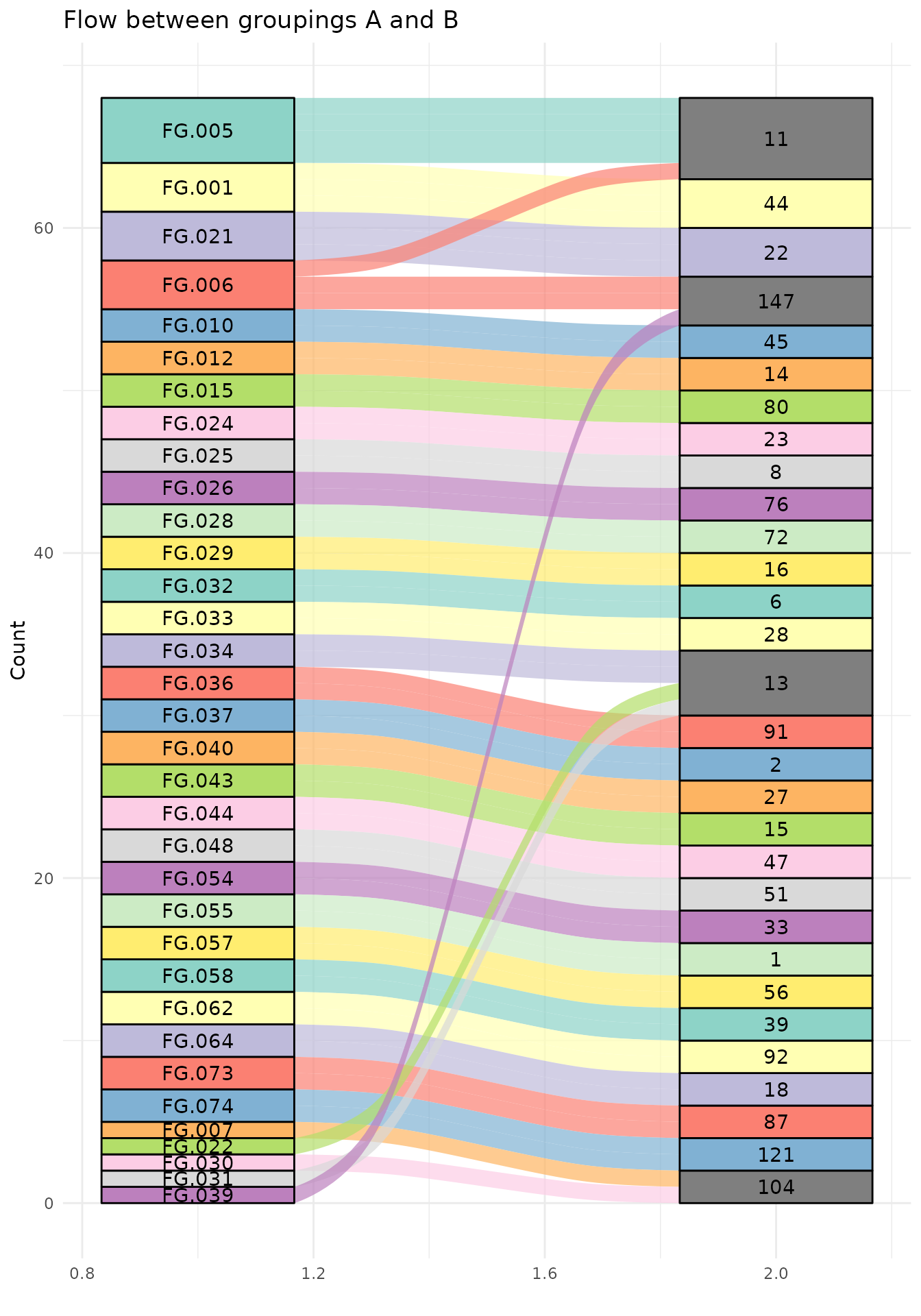

Or just look at those that are not mapped the same by CAMERA and groupFeatures.

group_mapping_different <- group_mapping %>%
  group_by(feature_group) %>%
  mutate(n_pc = n_distinct(pcgroup)) %>%
  group_by(pcgroup) %>%
  mutate(n_fg = n_distinct(feature_group)) %>%
  ungroup() %>%
  filter(n_pc > 1 | n_fg > 1)


ggplot(group_mapping_different, aes(axis1 = feature_group, axis2 = pcgroup, fill = feature_group)) +
  geom_alluvium(alpha = 0.7) +
  geom_stratum() +
  geom_text(stat = "stratum", aes(label = after_stat(stratum))) +
  theme_minimal() +
  labs(x = "", y = "Count", title = "Flow between groupings A and B") +
  guides(fill="none") +
  scale_fill_manual(values = rep(brewer.pal(12, "Set3"), length.out = length(unique(group_mapping_different$feature_group))))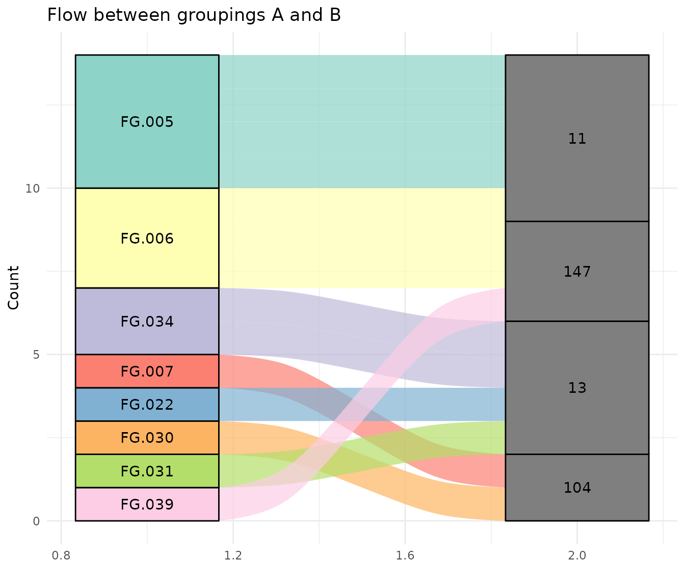

Understanding the Output

The resulting tibble contains comprehensive information about each feature in each sample. Below is a complete description of all columns:

Column Reference Table

The table has been organized into logical groups for easier understanding:

Column	Content
Sample information
filepath	Path to the raw data file
filename	The filename without path
fromFile	The file number (the order files were supplied in)
Plus any columns from sampleData()	Sample metadata columns (e.g., sample_name, sample_group, sample_type)
Feature identifiers
feature_id	The index of the feature after grouping across samples
peakidx	The index of the peak before grouping across samples
Feature-level m/z statistics (across all samples)
f_mzmed	The median m/z found for that feature across samples
f_mzmin	The minimum m/z found for that feature across samples
f_mzmax	The maximum m/z found for that feature across samples
Feature-level retention time statistics (across all samples)
f_rtmed	The median retention time found for that feature across samples
f_rtmin	The minimum retention time found for that feature across samples
f_rtmax	The maximum retention time found for that feature across samples
CAMERA annotations
isotopes	The isotope annotation from CAMERA (e.g., “[M]+”, “[M+1]+”, “[M+2]+”)
adduct	The adduct annotation from CAMERA (e.g., “[M+H]+”, “[M+Na]+”, “[M+NH4]+”)
pcgroup	The feature grouping index from CAMERA - features with same ID likely come from the same compound
MsFeatures annotations
feature_group	The feature group ID from MsFeatures (e.g., “FG.001”, “FG.002”) - features with same ID are grouped by retention time, abundance correlation, or EIC similarity
Peak-level m/z measurements (in that specific sample)
mz	The median m/z found for that feature in that sample
mzmin	The minimum m/z found for that feature in that sample
mzmax	The maximum m/z found for that feature in that sample
Peak-level retention time measurements (in that specific sample)
rt	The retention time found for that feature in that sample
rtmin	The minimum retention time found for that feature in that sample
rtmax	The maximum retention time found for that feature in that sample
Peak intensity measurements
into	The area under the peak
intb	The area under the peak after baseline removal
maxo	The maximum intensity (i.e., height) of the peak
sn	The signal to noise ratio of that peak
Gaussian peak fitting parameters
egauss	RMSE of Gaussian fit
mu	Gaussian parameter mu (center of the Gaussian; unit is scan number)
sigma	Gaussian parameter sigma
h	Gaussian parameter h (height of the Gaussian peak)
CentWave algorithm parameters
f	Region number of m/z ROI where the peak was localized
dppm	m/z deviation of mass trace across scans in ppm
scale	Scale on which the peak was localized
scpos	Center of peak position found by wavelet analysis
scmin	Left peak limit found by wavelet analysis (scan number)
scmax	Right peak limit found by wavelet analysis (scan number)
Additional columns
ms_level	MS level (e.g., MS1, MS2)
is_filled	Was the intensity found by gap filling (TRUE) or peak picking (FALSE)

Important notes:

• Each row represents one feature in one sample
• If a feature was not detected in a sample, peak-level columns (mz, rt, into, etc.) will be NA
• Feature-level statistics (f_mzmed, f_rtmed, etc.) are always present and represent values across all samples
• CAMERA annotations (isotopes, adduct, pcgroup) are optional and only present when xsAnnotate is provided
• MsFeatures annotations (feature_group) are optional and only present when groupFeatures() was applied
• Both CAMERA and MsFeatures annotations apply at the feature level and are the same across all samples for a given feature
• The distinction between “feature-level” and “peak-level” is important:
  • Feature-level (prefix f_): Statistics aggregated across all samples
  • Peak-level (no prefix): Values for the specific peak in that specific sample

Feature-Level Information

These columns describe each feature (grouped peak):

peak_table %>%
  select(feature_id, f_mzmed, f_rtmed) %>%
  distinct() %>%
  head()
#> # A tibble: 6 × 3
#>   feature_id f_mzmed f_rtmed
#>        <int>   <dbl>   <dbl>
#> 1          1    200.   2903.
#> 2          2    205    2790.
#> 3          3    206    2789.
#> 4          4    207.   2719.
#> 5          5    233    3024.
#> 6          6    241.   3683.

CAMERA Annotations

When CAMERA annotations are included, these additional columns are available:

• isotopes: Isotope annotation (e.g., “[M]+”, “[M+1]+”)
• adduct: Adduct annotation (e.g., “[M+H]+”, “[M+Na]+”)
• pcgroup: Pseudospectrum correlation group ID

# View features with adduct annotations (using the CAMERA-annotated table)
peak_table_camera %>%
  filter(adduct!="") %>%
  select(feature_id, f_mzmed, f_rtmed, isotopes, adduct, pcgroup) %>%
  distinct(feature_id, .keep_all = TRUE) %>%
  head()
#> # A tibble: 6 × 6
#>   feature_id f_mzmed f_rtmed isotopes  adduct                            pcgroup
#>        <int>   <dbl>   <dbl> <chr>     <chr>                               <int>
#> 1          3    206    2789. ""        [M+2K]2+ 334.047 [M+H-NH3-CO2-C5…      11
#> 2          6    241.   3683. ""        [M+H-S]+ 272.112 [M+H-CH3OH]+ 27…      87
#> 3         11    255.   3682. ""        [M+H-H2O]+ 272.112                     87
#> 4         13    266.   3669. ""        [M+H-C2H4-CO2]+ 337.215 [M+H-C4H…      44
#> 5         19    279    2788. ""        [M+H-C3H4O]+ 334.047 [M+H-C4H8]+…      11
#> 6         21    281.   3669. "[1][M]+" [M+H-NH3-C3H4]+ 337.215                44

Peak-Level Information

For each feature in each sample:

• mz, rt: Detected peak position
• into: Integrated peak intensity
• intb: Baseline-corrected intensity
• maxo: Maximum intensity
• sn: Signal-to-noise ratio

# View detected peaks (non-NA intensities)
peak_table %>%
  filter(!is.na(into)) %>%
  select(feature_id, filename, mz, rt, into, sn) %>%
  head()
#> # A tibble: 6 × 6
#>   feature_id filename    mz    rt     into    sn
#>        <int> <chr>    <dbl> <dbl>    <dbl> <dbl>
#> 1          1 ko15.CDF  200. 2933.  135162.    NA
#> 2          2 ko15.CDF  205  2792. 1924712.    64
#> 3          3 ko15.CDF  206  2790.  213659.    14
#> 4          4 ko15.CDF  207. 2718.  349011.    17
#> 5          5 ko15.CDF  233  3035.  286221.    23
#> 6          6 ko15.CDF  241. 3681. 1160580.    11

Sample Information

• filename, filepath: Sample file information
• fromFile: Sample index
• Plus any columns from sampleData() (sample metadata)

peak_table %>%
  select(feature_id, filename, sample_name, sample_group, sample_type) %>%
  head()
#> # A tibble: 6 × 5
#>   feature_id filename sample_name sample_group sample_type
#>        <int> <chr>    <chr>       <chr>        <chr>      
#> 1          1 ko15.CDF ko15        KO           QC         
#> 2          2 ko15.CDF ko15        KO           QC         
#> 3          3 ko15.CDF ko15        KO           QC         
#> 4          4 ko15.CDF ko15        KO           QC         
#> 5          5 ko15.CDF ko15        KO           QC         
#> 6          6 ko15.CDF ko15        KO           QC

Missing Values

Features not detected in a sample have NA for peak-level columns:

# Count for each feature how many samples the peak was found in
detection_rate <- peak_table %>%
  group_by(feature_id, f_mzmed, f_rtmed) %>%
  summarise(
    n_samples_detected = sum(!is.na(into)),
    n_samples_total = n(),
    detection_rate = n_samples_detected / n_samples_total,
    .groups = "drop"
  ) %>%
  arrange(desc(detection_rate))

hist(detection_rate$detection_rate, breaks=10, main = "Histogram of feature detection rate")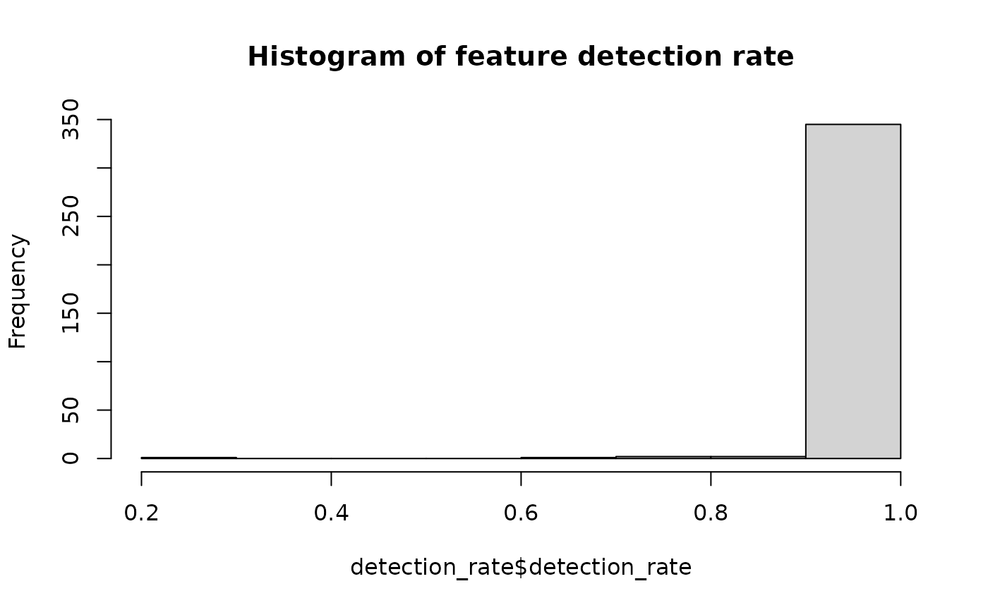

Downstream Analysis Examples

Visualize Feature Intensities

# Plot intensity distribution by sample group
peak_table %>%
  filter(feature_id == 10) %>%
  ggplot(aes(x = sample_group, y = log10(into), fill = sample_group)) +
  geom_boxplot() +
  labs(
    title = "Feature Intensity Distribution",
    x = "Sample Group",
    y = "log10(Intensity)"
  ) +
  theme_minimal()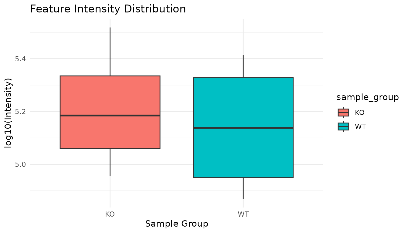

Identify Features with Adduct Annotations

# Count features by adduct type (using the CAMERA-annotated table)
adduct_counts <- peak_table_camera %>%
  filter(adduct!="") %>%
  separate_rows(adduct, sep = "\\s(?=\\[M)") %>%
  distinct(feature_id, adduct) %>%
  mutate(adduct = gsub("^(\\[.*\\].*\\+).*","\\1",adduct)) %>%

  count(adduct, sort = TRUE)

adduct_counts
#> # A tibble: 33 × 2
#>    adduct                  n
#>    <chr>               <int>
#>  1 [M+H]+                 12
#>  2 [M+Na]+                12
#>  3 [M+H-H2O]+             10
#>  4 [M+K]+                  6
#>  5 [M+H-C3H9N-C2H4O2]+     5
#>  6 [M+H-CH4]+              5
#>  7 [M+H-O]+                5
#>  8 [M+H-NH3]+              4
#>  9 [M+H-CH3OH]+            3
#> 10 [M+H-S]+                3
#> # ℹ 23 more rows

Visualize Adduct Distribution

We can create a pie chart showing the frequency of different adducts and fragments found by CAMERA:

# Create pie chart of adduct frequencies
adduct_counts %>% 
  mutate(count = n) %>% 
    ggpie(data = ., 
          group_key = "adduct", 
          count_type = "count",
          label_info = "group", 
          label_type = "circle",
          label_size = 4, 
          label_pos = "out"
          ) +
    guides(fill="none") +
    ggtitle("Distribution of Adduct Annotations")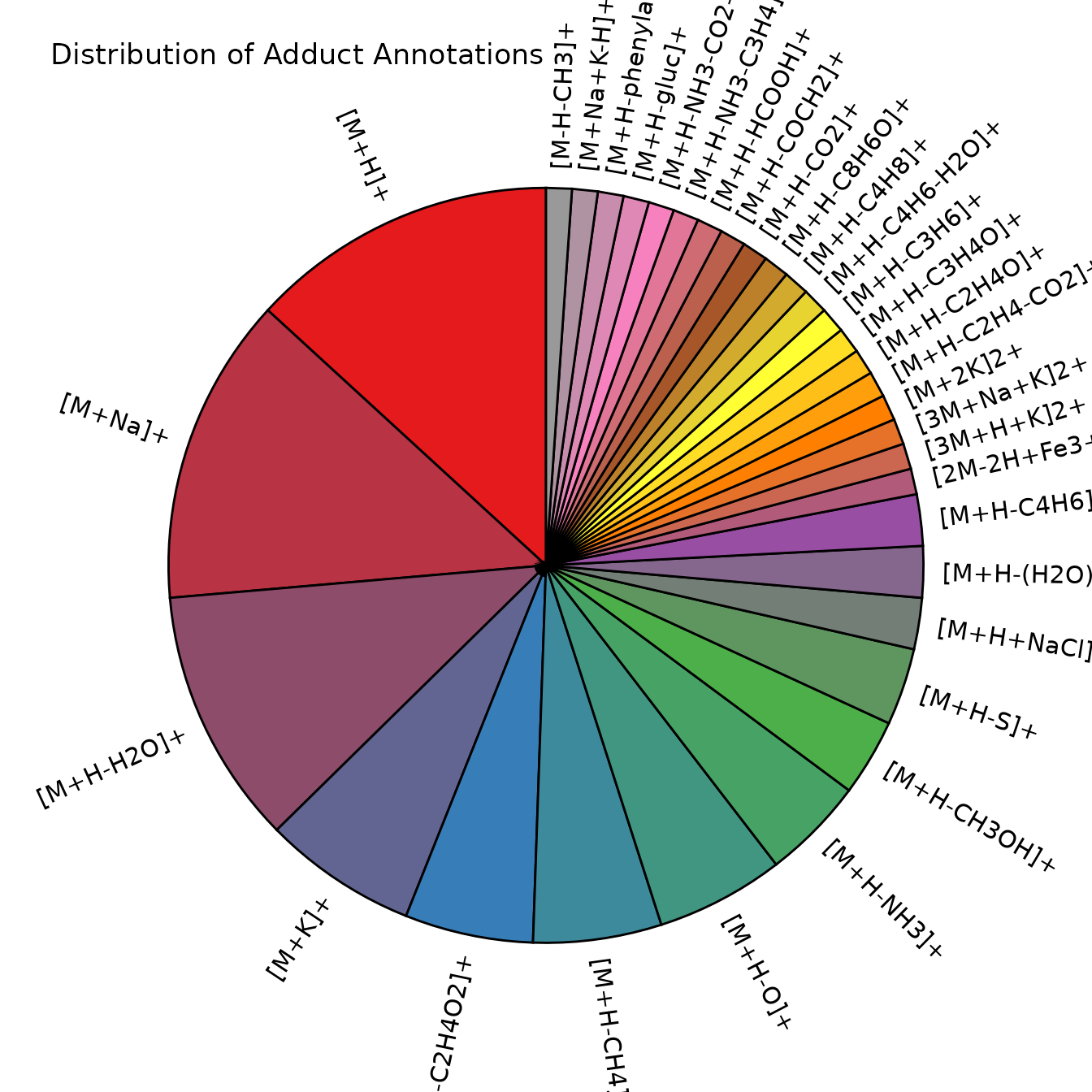

Extract Specific Features for Further Analysis

# Get a specific feature across all samples
feature_123 <- peak_table %>%
  filter(feature_id == 123) %>%
  select(feature_id, filename, sample_group, mz, rt, into)

head(feature_123)
#> # A tibble: 6 × 6
#>   feature_id filename sample_group    mz    rt    into
#>        <int> <chr>    <chr>        <dbl> <dbl>   <dbl>
#> 1        123 ko15.CDF KO            371. 3657. 563419.
#> 2        123 ko16.CDF KO            371. 3657. 320434.
#> 3        123 ko21.CDF KO            371. 3649. 123876.
#> 4        123 ko22.CDF KO            371. 3633. 173440.
#> 5        123 wt15.CDF WT            371. 3632. 570454.
#> 6        123 wt16.CDF WT            371. 3639. 287139.

Session Info

sessionInfo()
#> R version 4.5.2 (2025-10-31)
#> Platform: x86_64-pc-linux-gnu
#> Running under: Ubuntu 24.04.3 LTS
#> 
#> Matrix products: default
#> BLAS:   /usr/lib/x86_64-linux-gnu/openblas-pthread/libblas.so.3 
#> LAPACK: /usr/lib/x86_64-linux-gnu/openblas-pthread/libopenblasp-r0.3.26.so;  LAPACK version 3.12.0
#> 
#> locale:
#>  [1] LC_CTYPE=C.UTF-8       LC_NUMERIC=C           LC_TIME=C.UTF-8       
#>  [4] LC_COLLATE=C.UTF-8     LC_MONETARY=C.UTF-8    LC_MESSAGES=C.UTF-8   
#>  [7] LC_PAPER=C.UTF-8       LC_NAME=C              LC_ADDRESS=C          
#> [10] LC_TELEPHONE=C         LC_MEASUREMENT=C.UTF-8 LC_IDENTIFICATION=C   
#> 
#> time zone: UTC
#> tzcode source: system (glibc)
#> 
#> attached base packages:
#> [1] stats4    stats     graphics  grDevices utils     datasets  methods  
#> [8] base     
#> 
#> other attached packages:
#>  [1] ggpie_0.2.5         RColorBrewer_1.1-3  ggalluvial_0.12.5  
#>  [4] commonMZ_0.0.2      MsFeatures_1.18.0   CAMERA_1.66.0      
#>  [7] MSnbase_2.36.0      S4Vectors_0.48.0    mzR_2.44.0         
#> [10] Rcpp_1.1.0          Biobase_2.70.0      BiocGenerics_0.56.0
#> [13] generics_0.1.4      MsExperiment_1.12.0 ProtGenerics_1.42.0
#> [16] tidyr_1.3.1         ggplot2_4.0.0       dplyr_1.1.4        
#> [19] xcms_4.8.0          BiocParallel_1.44.0 tidyXCMS_0.99.37   
#> 
#> loaded via a namespace (and not attached):
#>   [1] rstudioapi_0.17.1           jsonlite_2.0.0             
#>   [3] MultiAssayExperiment_1.36.0 magrittr_2.0.4             
#>   [5] farver_2.1.2                MALDIquant_1.22.3          
#>   [7] rmarkdown_2.30              fs_1.6.6                   
#>   [9] ragg_1.5.0                  vctrs_0.6.5                
#>  [11] base64enc_0.1-3             htmltools_0.5.8.1          
#>  [13] S4Arrays_1.10.0             BiocBaseUtils_1.12.0       
#>  [15] progress_1.2.3              cellranger_1.1.0           
#>  [17] SparseArray_1.10.1          Formula_1.2-5              
#>  [19] mzID_1.48.0                 sass_0.4.10                
#>  [21] bslib_0.9.0                 htmlwidgets_1.6.4          
#>  [23] desc_1.4.3                  plyr_1.8.9                 
#>  [25] impute_1.84.0               cachem_1.1.0               
#>  [27] igraph_2.2.1                lifecycle_1.0.4            
#>  [29] iterators_1.0.14            pkgconfig_2.0.3            
#>  [31] Matrix_1.7-4                R6_2.6.1                   
#>  [33] fastmap_1.2.0               MatrixGenerics_1.22.0      
#>  [35] clue_0.3-66                 digest_0.6.38              
#>  [37] ggnewscale_0.5.2            pcaMethods_2.2.0           
#>  [39] colorspace_2.1-2            textshaping_1.0.4          
#>  [41] Hmisc_5.2-4                 GenomicRanges_1.62.0       
#>  [43] labeling_0.4.3              Spectra_1.20.0             
#>  [45] abind_1.4-8                 compiler_4.5.2             
#>  [47] bit64_4.6.0-1               withr_3.0.2                
#>  [49] doParallel_1.0.17           htmlTable_2.4.3            
#>  [51] S7_0.2.0                    backports_1.5.0            
#>  [53] DBI_1.2.3                   MASS_7.3-65                
#>  [55] DelayedArray_0.36.0         tools_4.5.2                
#>  [57] PSMatch_1.14.0              foreign_0.8-90             
#>  [59] nnet_7.3-20                 glue_1.8.0                 
#>  [61] QFeatures_1.20.0            grid_4.5.2                 
#>  [63] checkmate_2.3.3             cluster_2.1.8.1            
#>  [65] reshape2_1.4.5              gtable_0.3.6               
#>  [67] tzdb_0.5.0                  preprocessCore_1.72.0      
#>  [69] data.table_1.17.8           hms_1.1.4                  
#>  [71] MetaboCoreUtils_1.18.0      utf8_1.2.6                 
#>  [73] XVector_0.50.0              ggrepel_0.9.6              
#>  [75] foreach_1.5.2               pillar_1.11.1              
#>  [77] stringr_1.6.0               vroom_1.6.6                
#>  [79] limma_3.66.0                lattice_0.22-7             
#>  [81] bit_4.6.0                   tidyselect_1.2.1           
#>  [83] RBGL_1.86.0                 knitr_1.50                 
#>  [85] gridExtra_2.3               IRanges_2.44.0             
#>  [87] Seqinfo_1.0.0               SummarizedExperiment_1.40.0
#>  [89] xfun_0.54                   statmod_1.5.1              
#>  [91] matrixStats_1.5.0           stringi_1.8.7              
#>  [93] lazyeval_0.2.2              yaml_2.3.10                
#>  [95] evaluate_1.0.5              codetools_0.2-20           
#>  [97] MsCoreUtils_1.21.0          tibble_3.3.0               
#>  [99] BiocManager_1.30.26         graph_1.88.0               
#> [101] cli_3.6.5                   affyio_1.80.0              
#> [103] rpart_4.1.24                systemfonts_1.3.1          
#> [105] jquerylib_0.1.4             MassSpecWavelet_1.76.0     
#> [107] readxl_1.4.5                XML_3.99-0.20              
#> [109] parallel_4.5.2              pkgdown_2.2.0              
#> [111] readr_2.1.5                 prettyunits_1.2.0          
#> [113] AnnotationFilter_1.34.0     scales_1.4.0               
#> [115] affy_1.88.0                 ncdf4_1.24                 
#> [117] purrr_1.2.0                 crayon_1.5.3               
#> [119] rlang_1.1.6                 vsn_3.78.0