ggplot2 Version of plot() for XChromatogram

Creates a ggplot2 version of a chromatogram with detected peaks marked. This is equivalent to the base R plot() method for XChromatogram objects.

Creates a ggplot2 version of the retention time alignment model visualization for xcms::LamaParama() objects. LamaParama objects contain parameters and results from landmark-based retention time alignment.

Usage

gplot(x, ...)

# S4 method for class 'LamaParama'
gplot(x, index = 1L, colPoints = "#00000060", colFit = "#00000080", ...)

# S4 method for class 'XChromatogram'
gplot(
  x,
  col = "black",
  lty = 1,
  type = "l",
  peakType = c("polygon", "point", "rectangle", "none"),
  peakCol = "#00000060",
  peakBg = "#00000020",
  peakPch = 1,
  ...
)

# S4 method for class 'XChromatograms'
gplot(
  x,
  col = "#00000060",
  lty = 1,
  type = "l",
  peakType = c("polygon", "point", "rectangle", "none"),
  peakCol = "#00000060",
  peakBg = "#00000020",
  peakPch = 1,
  include_columns = NULL,
  ...
)

# S4 method for class 'MChromatograms'
gplot(
  x,
  col = "#00000060",
  lty = 1,
  type = "l",
  peakType = c("polygon", "point", "rectangle", "none"),
  peakCol = "#00000060",
  peakBg = "#00000020",
  peakPch = 1,
  include_columns = NULL,
  ...
)

Arguments

x: A LamaParama object containing retention time alignment parameters and results.
...: Additional parameters (currently unused, for S4 compatibility).
index: integer(1) specifying which retention time map to plot (default: 1).
colPoints: Color for the matched peak points (default: semi-transparent black).
colFit: Color for the fitted model line (default: semi-transparent black).
col: Color for the chromatogram line (default: "black"). For XChromatograms and MChromatograms objects, this can also be a column name from pData(x) to map color to sample metadata (e.g., col = "sample_group"). When a column name is used, ggplot2 automatically adds a color legend.
lty: Line type for chromatogram (default: 1).
type: Plot type (default: "l" for line).
peakType: character(1) defining the type of peak annotation: "polygon", "point", "rectangle", or "none" (default: "polygon").
peakCol: Color for peak markers (default: "#00000060"). For XChromatograms objects, this can also be a column name from pData(x) to map peak border color to sample metadata.
peakBg: Background color for peak markers (default: "#00000020"). For XChromatograms objects, this can also be a column name from pData(x) to map peak fill color to sample metadata.
peakPch: Point character for peak markers when peakType = "point" (default: 1).
include_columns: For XChromatograms and MChromatograms: which pData(x) columns to include in plotly tooltips. NULL (default) for no metadata in tooltips, TRUE for all columns, or a character vector of specific column names. The tooltip text is stored in the text aesthetic and is used by plotly::ggplotly().

Value

A ggplot object.

Details

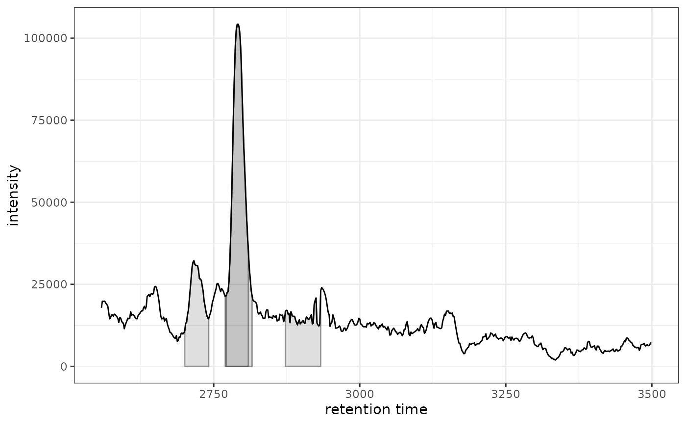
This function creates a complete chromatogram plot with detected peaks automatically marked, similar to the base R plot() method for XChromatogram objects. If the chromatogram contains detected peaks, they will be shown according to the peakType parameter.

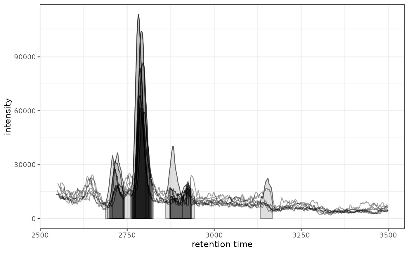
Color Mapping for Multi-Sample Chromatograms

When plotting XChromatograms or MChromatograms objects (multiple samples), the col, peakCol, and peakBg parameters accept either:

A static color string (e.g., col = "red", col = "#00000060") — all samples use the same color (default behavior).
A column name from pData(x) as a quoted string (e.g., col = "sample_group") — each sample is colored according to its metadata value. The column must exist in Biobase::pData(x), which inherits from sampleData() of the parent XcmsExperiment object. The value is automatically detected as a column name when it matches a column in pData(x).

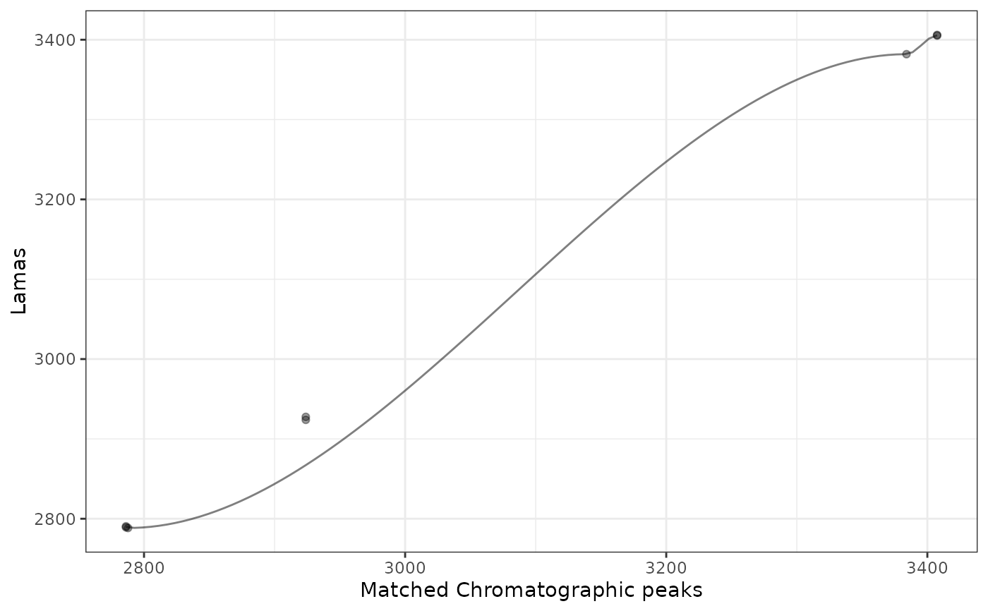
This function visualizes the retention time alignment model for a specific sample.

The plot shows:

Points representing matched chromatographic peaks between the sample and reference
A fitted line (loess or GAM) showing the retention time correction model

The LamaParama object contains parameters for landmark-based alignment including:

method: The fitting method ("loess" or "gam")
span: Span parameter for loess fitting
outlierTolerance: Tolerance for outlier detection
zeroWeight: Weight for the (0,0) anchor point
bs: Basis function for GAM fitting
rtMap: List of data frames with retention time pairs

Author

Jan Stanstrup

Examples

library(xcmsVis)
library(xcms)
library(faahKO)
library(MsExperiment)
library(ggplot2)

## Load preprocessed data
xdata <- loadXcmsData()
# Extract chromatogram
chr <- chromatogram(xdata, mz = c(200, 210), rt = c(2500, 3500))
#> Extracting chromatographic data
#> Processing chromatographic peaks
#> Processing features

# Plot with ggplot2
gplot(chr[1, 1])
#> Warning: Ignoring unknown aesthetics: text


# Plot data for all samples
gplot(chr)
#> Warning: Ignoring unknown aesthetics: text


# Color by sample metadata (requires pData column)
# gplot(chr, col = "sample_group")


library(xcmsVis)
library(xcms)
library(MsExperiment)

# LamaParama requires a reference dataset with landmarks
# See vignette("04-retention-time-alignment") for complete workflow

# Load reference and test datasets
ref <- loadXcmsData("xmse")
tst <- loadXcmsData("faahko_sub2")

# Extract landmarks from QC samples in reference
f <- sampleData(ref)$sample_type
f[f != "QC"] <- NA
ref_filtered <- filterFeatures(
    ref, PercentMissingFilter(threshold = 0, f = f))
#> 4 features were removed
ref_mz_rt <- featureDefinitions(ref_filtered)[, c("mzmed", "rtmed")]

# Create and apply LamaParama alignment
lama_param <- LamaParama(lamas = ref_mz_rt, method = "loess", span = 0.5)
tst_adjusted <- adjustRtime(tst, param = lama_param)

# Extract LamaParama result for visualization
proc_hist <- processHistory(tst_adjusted,
    type = xcms:::.PROCSTEP.RTIME.CORRECTION)
lama_result <- proc_hist[[length(proc_hist)]]@param

# Visualize the first sample's alignment
gplot(lama_result, index = 1)
#> Warning: pseudoinverse used at -17.037
#> Warning: neighborhood radius 2804.8
#> Warning: reciprocal condition number  0
#> Warning: There are other near singularities as well. 2.5061e+05
#> Warning: span too small.   fewer data values than degrees of freedom.
#> Warning: pseudoinverse used at -17.037
#> Warning: neighborhood radius 2803.2
#> Warning: reciprocal condition number  0
#> Warning: There are other near singularities as well. 1641.2

ggplot2 Version of `plot()` for `XChromatogram`