library(xcms)
library(xcmsVis)
library(MsExperiment)
library(MsFeatures)
library(ggplot2)
library(BiocParallel)
library(patchwork)
# Configure for serial processing
register(SerialParam())Introduction
This vignette covers the final step in the xcms metabolomics workflow: feature grouping. After retention time alignment, these functions help you:
- Visualize relationships between features
- Identify isotopes, adducts, and fragments
- Assess feature annotation quality
- Create publication-ready feature network plots
xcms Workflow Context
┌───────────────────────────────┐
│ 1. Raw Data Visualization     │
│ 2. Peak Detection             │
│ 3. Peak Correspondence        │
│ 4. Retention Time Alignment   │
├───────────────────────────────┤
│ 5. FEATURE GROUPING           │ ← YOU ARE HERE
└───────────────────────────────┘
What is Feature Grouping?
Feature grouping identifies features that likely represent the same compound. After feature detection and correspondence, groupFeatures() connects features that may be:
- Isotopes: M+1, M+2 isotopic peaks
- Adducts: [M+H]+, [M+Na]+, [M+K]+, etc.
- Fragments: In-source fragmentation products
- Correlated features: Compounds with similar abundance patterns
The gplotFeatureGroups() function visualizes these relationships by plotting features connected by lines within each group across retention time and m/z dimensions.
Functions Covered
| Function | Purpose | Input |
|---|---|---|
gplotFeatureGroups() |
Visualize feature group relationships |
XcmsExperiment, XCMSnExp
|
Setup
Load and Process Data
Feature grouping requires a complete xcms workflow: peak detection, correspondence, retention time alignment, re-correspondence, and then feature grouping.
We’ll use pre-processed data with peaks already detected:
# Load pre-processed data with detected peaks
# This dataset contains 248 detected peaks from 3 samples
xdata <- loadXcmsData("faahko_sub2")

# Add sample metadata
sampleData(xdata)$sample_name <- c("KO01", "KO02", "WT01")
sampleData(xdata)$sample_group <- c("KO", "KO", "WT")

cat("Loaded", length(fileNames(xdata)), "files\n")
#> Loaded 3 files
cat("Detected peaks:", nrow(chromPeaks(xdata)), "\n")
#> Detected peaks: 248
Complete XCMS Workflow
# 1. Peak grouping (correspondence)
pdp <- PeakDensityParam(sampleGroups = sampleData(xdata)$sample_group,
                        minFraction = 0.5, bw = 30)
xdata <- groupChromPeaks(xdata, param = pdp)
cat("Grouped into", nrow(featureDefinitions(xdata)), "features\n")
#> Grouped into 152 features

# 2. Retention time alignment
xdata <- adjustRtime(xdata, param = ObiwarpParam())

# 3. Re-group after alignment
xdata <- groupChromPeaks(xdata, param = pdp)
cat("After alignment:", nrow(featureDefinitions(xdata)), "features\n")
#> After alignment: 152 features

# 4. Group features (identify related features)
xdata <- groupFeatures(xdata, param = SimilarRtimeParam(diffRt = 20))
cat("Identified", length(unique(featureGroups(xdata))), "feature groups\n")
#> Identified 63 feature groups
Basic Feature Group Visualization
The default plot shows all feature groups, with features connected by lines within each group:
gplotFeatureGroups(xdata)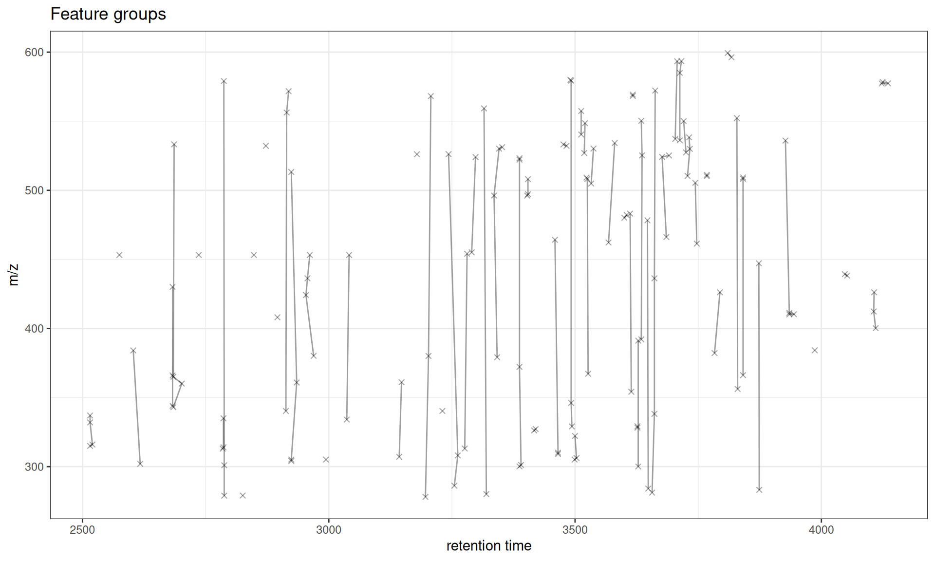
Interpretation
- Points: Individual features (at their median RT and m/z across samples)
- Lines: Connect features within the same group
- Groups: Represent features likely from the same compound (isotopes, adducts, etc.)
Filtering to Specific Feature Groups
You can visualize specific feature groups of interest:
# Get all feature group IDs
all_groups <- unique(featureGroups(xdata))
cat("Feature groups:", head(all_groups, 10), "\n")
#> Feature groups: FG.043 FG.012 FG.054 FG.038 FG.019 FG.023 FG.028 FG.048 FG.009 FG.018

# Plot first 5 groups
gplotFeatureGroups(xdata, featureGroups = all_groups[1:5]) +
  ggtitle("First 5 Feature Groups")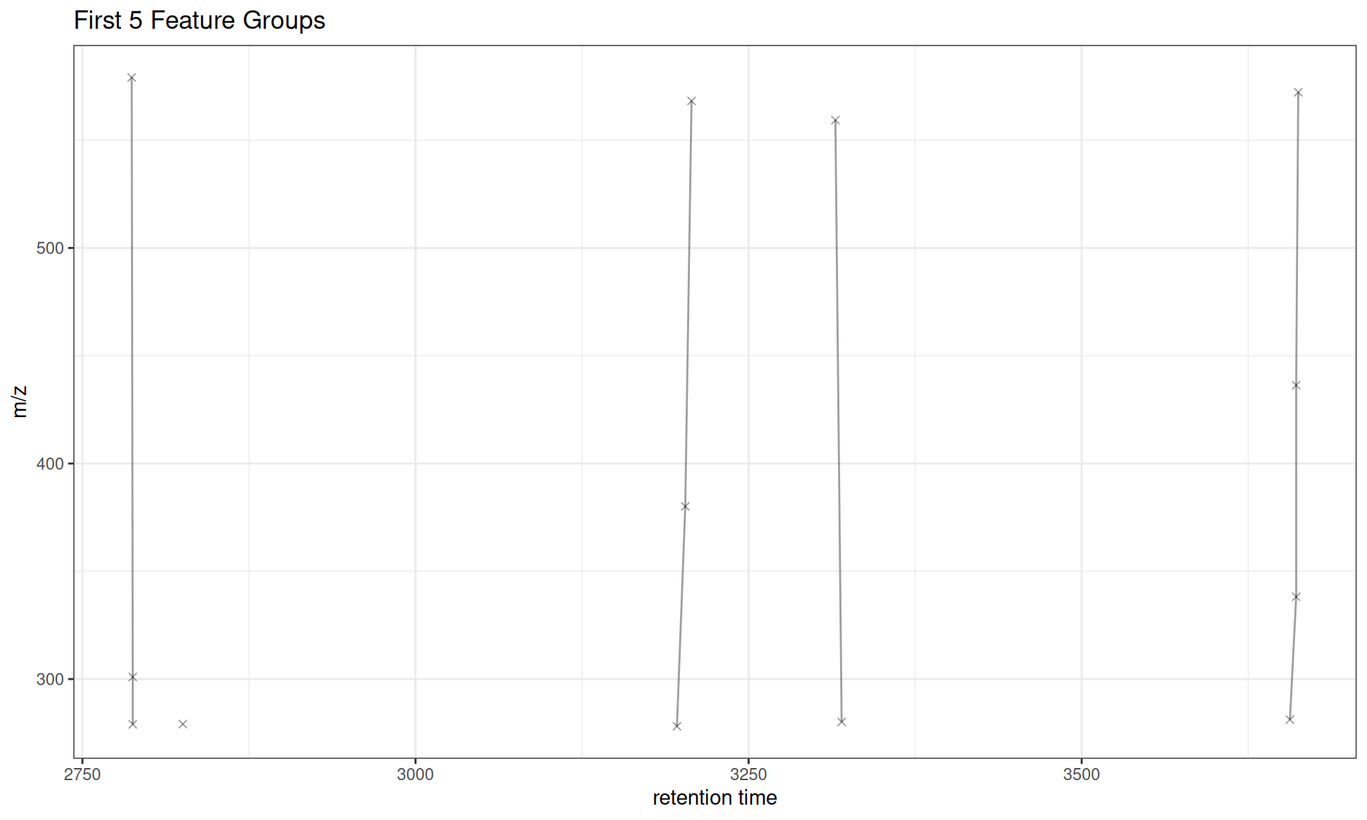
Customization
Custom Styling
# Get first 5 feature groups for clearer visualization
all_groups <- unique(featureGroups(xdata))

gplotFeatureGroups(xdata,
                   featureGroups = all_groups[1:5],
                   col = "#E31A1C",  # Red color
                   pch = 16) +       # Solid circles
  labs(x = "Retention Time (sec)",
       y = "Mass-to-Charge Ratio (m/z)",
       title = "Custom Styled Feature Groups")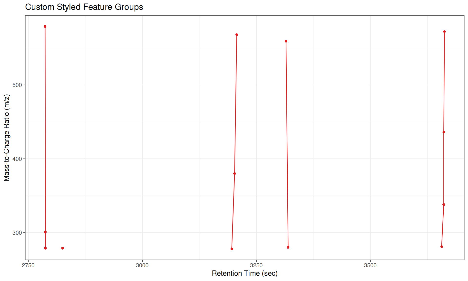
Different Plot Types
The type parameter controls whether to show lines, points, or both:
# Use subset of feature groups for clearer visualization
fg_subset <- all_groups[1:5]

# Plot with lines and points (default)
p1 <- gplotFeatureGroups(xdata, featureGroups = fg_subset, type = "o") +
  ggtitle('type = "o" (overplot - lines + points)')

# Plot with lines only
p2 <- gplotFeatureGroups(xdata, featureGroups = fg_subset, type = "l") +
  ggtitle('type = "l" (lines only)')

# Plot with points only
p3 <- gplotFeatureGroups(xdata, featureGroups = fg_subset, type = "p", pch = 16) +
  ggtitle('type = "p" (points only)')

# Combine plots
p1 / p2 / p3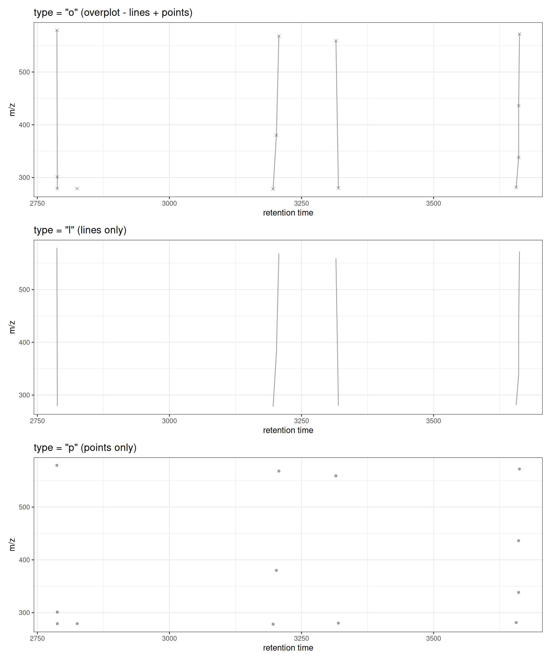
Zooming to Specific Regions
Use xlim and ylim to focus on specific retention time or m/z ranges:
# Focus on features between 3200-3300 seconds RT and specific feature groups
gplotFeatureGroups(xdata,
                   featureGroups = fg_subset,
                   xlim = c(3100, 3400),
                   ylim = c(200, 600)) +
  ggtitle("Features in RT 3200-3300 sec, m/z 200-600")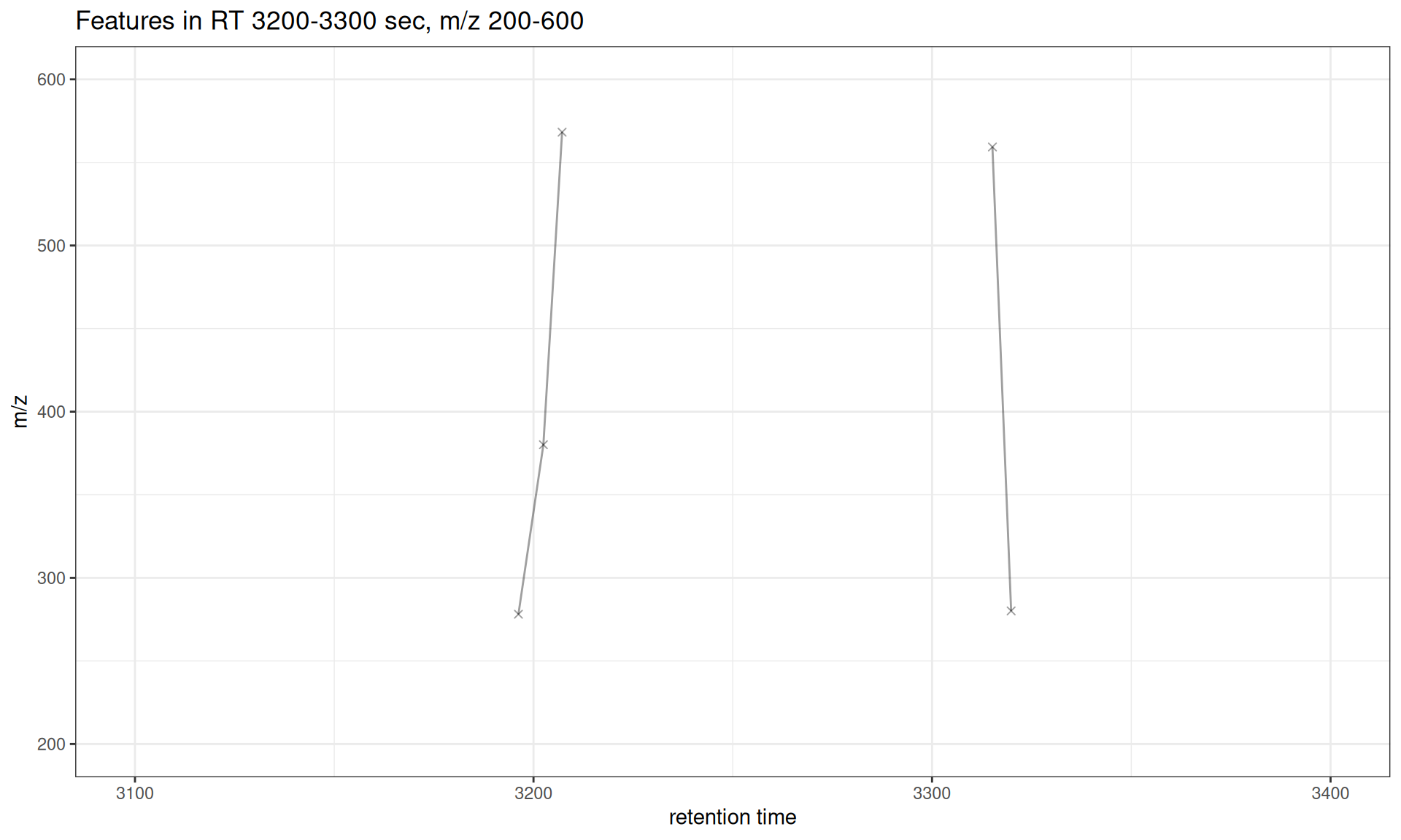
Interactive Visualization
Convert to interactive plotly plot for exploration:
library(plotly)

# Use subset for better interactivity
p <- gplotFeatureGroups(xdata, featureGroups = fg_subset)
ggplotly(p)
Understanding Feature Groups
Feature groups represent features that are likely derived from the same compound. Common grouping parameters:
Similar Retention Time
# Group features with similar retention times (likely isotopes/adducts)
xdata_rt <- groupFeatures(xdata, param = SimilarRtimeParam(diffRt = 10))
cat("SimilarRtimeParam (diffRt=10):",
    length(unique(featureGroups(xdata_rt))), "groups\n")
#> SimilarRtimeParam (diffRt=10): 76 groups

# Show first 5 groups
fg_rt <- unique(featureGroups(xdata_rt))
gplotFeatureGroups(xdata_rt, featureGroups = fg_rt[1:5]) +
  ggtitle("Feature Groups: Similar Retention Time (diffRt = 10 sec)")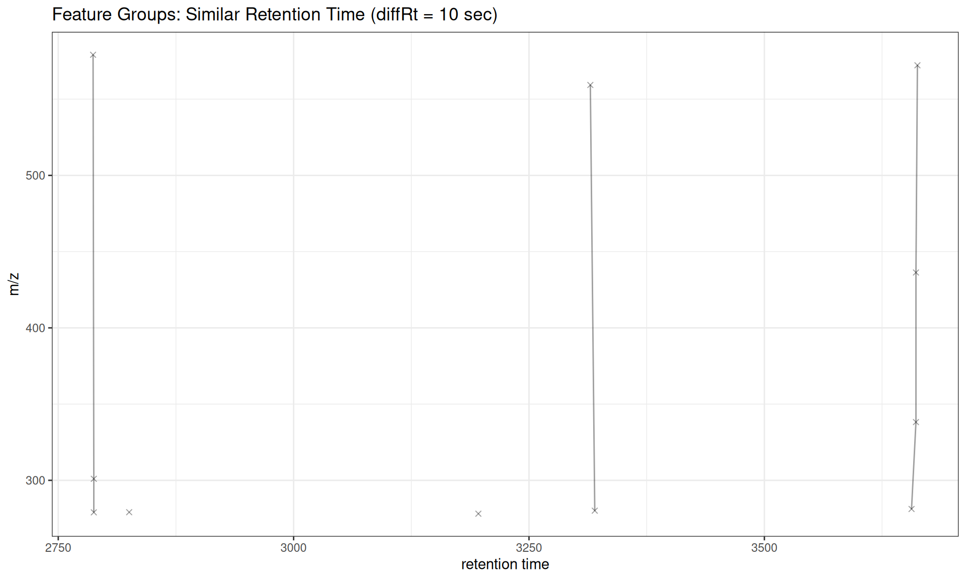
Abundance Correlation
# Group features with correlated abundances across samples
xdata_cor <- groupFeatures(
    xdata, param = AbundanceSimilarityParam(threshold = 0.7))
cat("AbundanceSimilarityParam (threshold=0.7):",
    length(unique(featureGroups(xdata_cor))), "groups\n")
#> AbundanceSimilarityParam (threshold=0.7): 139 groups

# Show some groups with multiple Features
fg_cor <- names(rev(sort(table(featureGroups(xdata_cor)))))
gplotFeatureGroups(xdata_cor, featureGroups = fg_cor[1:5]) +
  ggtitle("Feature Groups: Abundance Correlation (threshold = 0.7)")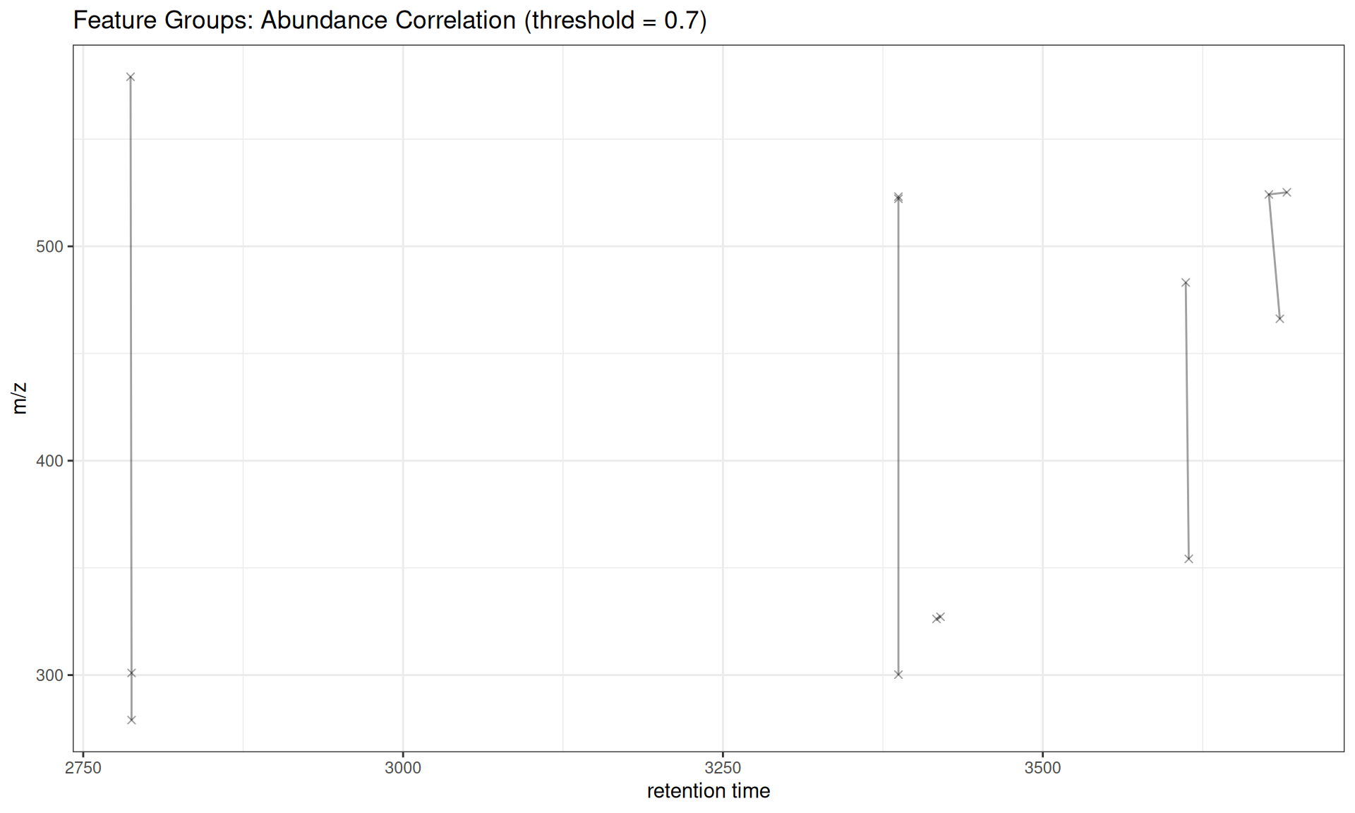
Use Cases
Isotope Pattern Identification
Features grouped by similar RT and abundance correlation may represent isotope patterns (e.g. M, M+1, M+2) or adducts (e.g. [M+H]+, [M+Na]+).
Adduct Identification
Features with similar RT but different m/z values that correlate in abundance may be different adducts of the same compound.
Quality Control
Visualize feature groups to:
- Verify grouping parameters are appropriate
- Identify over-grouping (too many features in one group)
- Identify under-grouping (features that should be grouped but aren’t)
Summary
Use Cases
- Compound annotation: Identify isotopes, adducts, and fragments
- Quality control: Verify feature grouping quality
- Method development: Optimize groupFeatures parameters
- Publication: Create network plots of feature relationships
Workflow Complete!
You’ve now completed the full xcms visualization workflow:
✓ 1. Raw Data Visualization
✓ 2. Peak Detection
✓ 3. Peak Correspondence
✓ 4. Retention Time Alignment
✓ 5. Feature Grouping
Comparison with Original xmcs
Original xcms Version
# Get first 5 feature groups for comparison
fg_compare <- unique(featureGroups(xdata))[1:5]

# XCMS original (base R graphics)
plotFeatureGroups(xdata, featureGroups = fg_compare)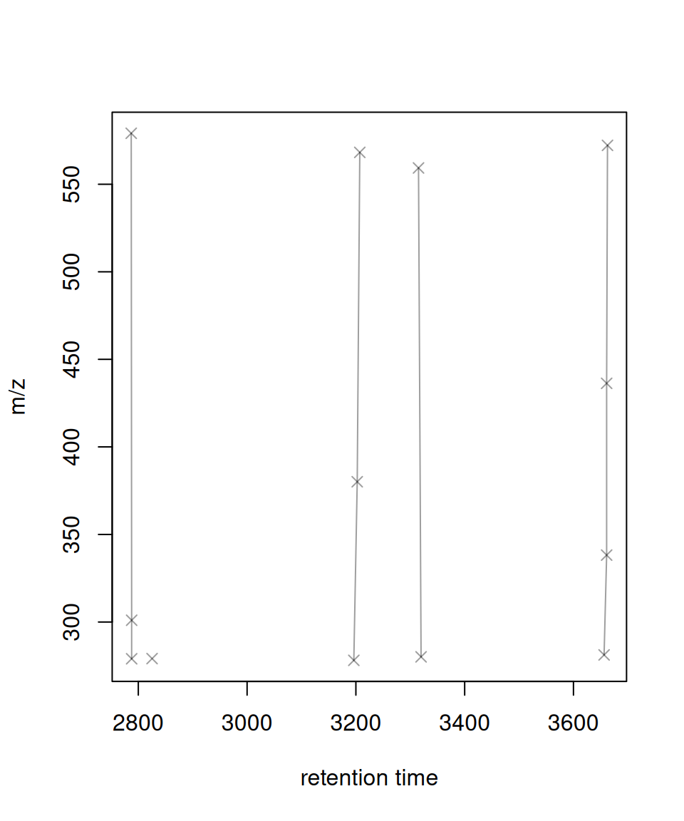
xcmsVis ggplot2 Version
# xcmsVis version (ggplot2)
gplotFeatureGroups(xdata, featureGroups = fg_compare)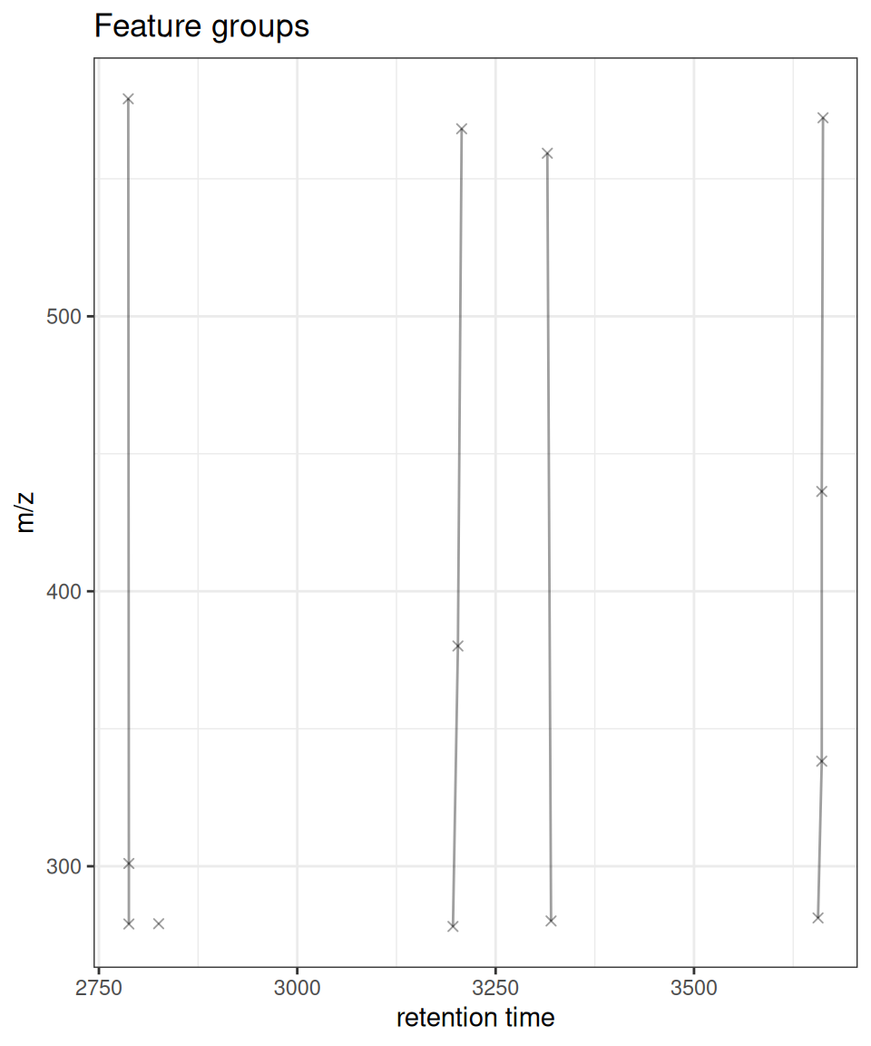
API Differences
Unlike the original xcms
plotFeatureGroups(), the ggplot2 version does not havexlab,ylab, ormainparameters. Instead, use ggplot2’slabs()function to customize labels after plot creation:# Customize labels with labs() fg_subset <- unique(featureGroups(xdata))[1:2] gplotFeatureGroups(xdata, featureGroups = fg_subset) + labs(x = "Retention Time (s)", y = "Mass/Charge", title = "My Custom Title")This follows ggplot2 conventions and makes the API more consistent with the broader ggplot2 ecosystem.
Session Info
sessionInfo()
#> R version 4.6.0 (2026-04-24)
#> Platform: x86_64-pc-linux-gnu
#> Running under: Ubuntu 24.04.4 LTS
#>
#> Matrix products: default
#> BLAS:   /usr/lib/x86_64-linux-gnu/openblas-pthread/libblas.so.3
#> LAPACK: /usr/lib/x86_64-linux-gnu/openblas-pthread/libopenblasp-r0.3.26.so;  LAPACK version 3.12.0
#>
#> locale:
#>  [1] LC_CTYPE=C.UTF-8       LC_NUMERIC=C           LC_TIME=C.UTF-8
#>  [4] LC_COLLATE=C.UTF-8     LC_MONETARY=C.UTF-8    LC_MESSAGES=C.UTF-8
#>  [7] LC_PAPER=C.UTF-8       LC_NAME=C              LC_ADDRESS=C
#> [10] LC_TELEPHONE=C         LC_MEASUREMENT=C.UTF-8 LC_IDENTIFICATION=C
#>
#> time zone: UTC
#> tzcode source: system (glibc)
#>
#> attached base packages:
#> [1] stats     graphics  grDevices utils     datasets  methods   base
#>
#> other attached packages:
#> [1] plotly_4.12.0       patchwork_1.3.2     ggplot2_4.0.3
#> [4] MsFeatures_1.20.0   MsExperiment_1.14.0 ProtGenerics_1.44.0
#> [7] xcmsVis_0.99.11     xcms_4.10.0         BiocParallel_1.46.0
#>
#> loaded via a namespace (and not attached):
#>   [1] DBI_1.3.0                   rlang_1.2.0
#>   [3] magrittr_2.0.5              clue_0.3-68
#>   [5] MassSpecWavelet_1.78.0      otel_0.2.0
#>   [7] matrixStats_1.5.0           compiler_4.6.0
#>   [9] PTMods_1.0.0                vctrs_0.7.3
#>  [11] reshape2_1.4.5              stringr_1.6.0
#>  [13] pkgconfig_2.0.3             MetaboCoreUtils_1.20.1
#>  [15] crayon_1.5.3                fastmap_1.2.0
#>  [17] XVector_0.52.0              labeling_0.4.3
#>  [19] rmarkdown_2.31              preprocessCore_1.74.0
#>  [21] purrr_1.2.2                 xfun_0.57
#>  [23] MultiAssayExperiment_1.38.0 jsonlite_2.0.0
#>  [25] progress_1.2.3              DelayedArray_0.38.1
#>  [27] parallel_4.6.0              prettyunits_1.2.0
#>  [29] cluster_2.1.8.2             R6_2.6.1
#>  [31] stringi_1.8.7               RColorBrewer_1.1-3
#>  [33] limma_3.68.1                GenomicRanges_1.64.0
#>  [35] Rcpp_1.1.1-1.1              Seqinfo_1.2.0
#>  [37] SummarizedExperiment_1.42.0 iterators_1.0.14
#>  [39] knitr_1.51                  IRanges_2.46.0
#>  [41] Matrix_1.7-5                igraph_2.3.1
#>  [43] tidyselect_1.2.1            abind_1.4-8
#>  [45] yaml_2.3.12                 doParallel_1.0.17
#>  [47] codetools_0.2-20            affy_1.90.0
#>  [49] lattice_0.22-9              tibble_3.3.1
#>  [51] plyr_1.8.9                  withr_3.0.2
#>  [53] Biobase_2.72.0              S7_0.2.2
#>  [55] evaluate_1.0.5              Spectra_1.22.0
#>  [57] pillar_1.11.1               affyio_1.82.0
#>  [59] BiocManager_1.30.27         MatrixGenerics_1.24.0
#>  [61] foreach_1.5.2               stats4_4.6.0
#>  [63] MSnbase_2.37.0              MALDIquant_1.22.3
#>  [65] ncdf4_1.24                  generics_0.1.4
#>  [67] S4Vectors_0.50.0            hms_1.1.4
#>  [69] scales_1.4.0                glue_1.8.1
#>  [71] lazyeval_0.2.3              tools_4.6.0
#>  [73] mzID_1.50.0                 data.table_1.18.2.1
#>  [75] QFeatures_1.22.0            vsn_3.80.0
#>  [77] mzR_2.46.0                  fs_2.1.0
#>  [79] XML_3.99-0.23               grid_4.6.0
#>  [81] impute_1.86.0               tidyr_1.3.2
#>  [83] crosstalk_1.2.2             MsCoreUtils_1.24.0
#>  [85] PSMatch_1.16.0              cli_3.6.6
#>  [87] viridisLite_0.4.3           S4Arrays_1.12.0
#>  [89] dplyr_1.2.1                 AnnotationFilter_1.36.0
#>  [91] pcaMethods_2.4.0            gtable_0.3.6
#>  [93] digest_0.6.39               BiocGenerics_0.58.0
#>  [95] SparseArray_1.12.2          htmlwidgets_1.6.4
#>  [97] farver_2.1.2                htmltools_0.5.9
#>  [99] lifecycle_1.0.5             httr_1.4.8
#> [101] statmod_1.5.1               MASS_7.3-65