ggplot2 Version of plot() for MsExperiment, XcmsExperiment and XCMSnExp
Source: R/gplot-XcmsExperiment-methods.R
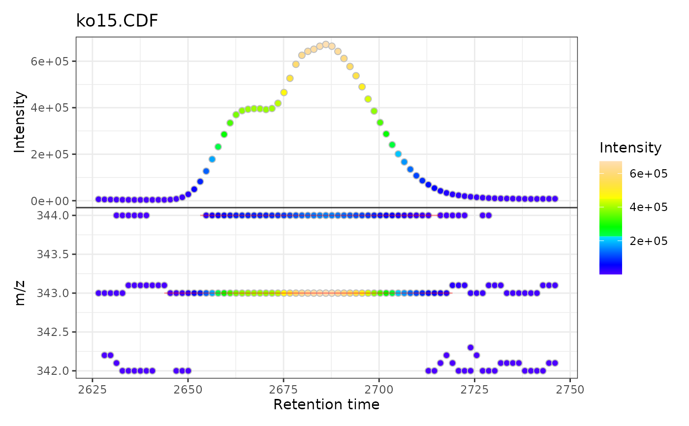
gplot-XcmsExperiment.RdCreates a two-panel visualization of MS data showing:
Upper panel: Base Peak Intensity (BPI) chromatogram vs retention time
Lower panel: m/z vs retention time scatter plot with intensity-based coloring
This is a ggplot2 implementation of xcms's plot() method for
MsExperiment objects, enabling modern visualization and interactive
plotting capabilities.
Usage
# S4 method for class 'XcmsExperiment'
gplot(
  x,
  msLevel = 1L,
  peakCol = "#ff000060",
  col = "grey",
  colramp = grDevices::topo.colors,
  pch = 21,
  ...
)

# S4 method for class 'MsExperiment'
gplot(
  x,
  msLevel = 1L,
  col = "grey",
  colramp = grDevices::topo.colors,
  pch = 21,
  ...
)

# S4 method for class 'XCMSnExp'
gplot(
  x,
  msLevel = 1L,
  peakCol = "#ff000060",
  col = "grey",
  colramp = grDevices::topo.colors,
  pch = 21,
  ...
)
Arguments
- x
MsExperiment,XcmsExperimentorXCMSnExpobject- msLevel
integer(1)defining the MS level to visualize (default:1)- peakCol
character(1)color to indicate identified chromatographic peaks (default:"#ff000060")- col
character(1)color for point borders (default:"grey")- colramp
function color ramp for intensity mapping (default:
grDevices::topo.colors)- pch
integer(1)point shape (default:21= filled circle)- ...
additional arguments (for compatibility)
Value
A ggplot or patchwork object showing the two-panel visualization.
For single samples, returns a patchwork object with two panels.
For multiple samples, returns a patchwork object with all sample plots
stacked. Use + labs() to customize axis labels and titles.
Details
The function:
Extracts spectra data filtered by MS level
Applies adjusted retention times if available
Upper panel: plots BPI (max intensity per retention time) with intensity-colored points
Lower panel: plots m/z vs retention time scatter with intensity-colored points
Overlays detected chromatographic peaks as rectangles (if available)
Uses consistent color scale across both panels based on intensity
See also
plot,MsExperiment,missing-method for the original
xcms implementation
Examples
library(xcmsVis)
library(xcms)
library(MsExperiment)
# Load and filter data
xmse <- loadXcmsData()
xmse <- filterRt(xmse, rt = c(2620, 2740)) |>
filterMzRange(mz = c(342, 344))
#> Filter spectra
#> Filter spectra
# Plot MS data
gplot(xmse[1L])
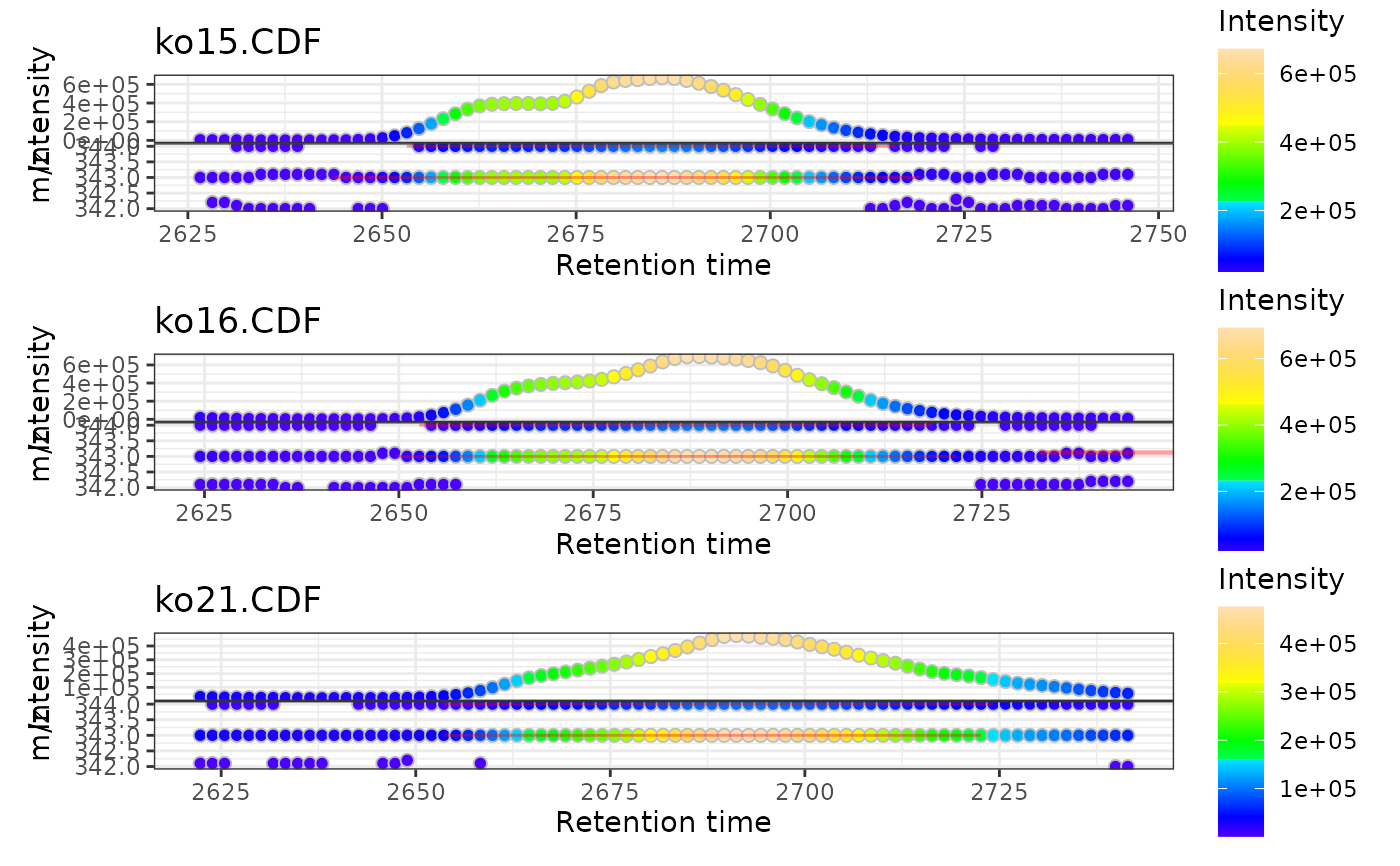
 # Multiple samples
gplot(xmse[1:3])
# Multiple samples
gplot(xmse[1:3])