5  ggplot2 Themes

5.1 Introduction

The default gray background theme in ggplot2 is iconic but completely inappropriate for publication. This chapter shows you the professional themes you should use instead, how to set a global theme for consistency, and which packages provide ready-made publication-quality themes.

Learning Objectives

By the end of this chapter, you will:

• Understand why theme_gray() is unsuitable for publications
• Know the best built-in themes: theme_classic(), theme_bw(), theme_minimal()
• Learn to set a global theme with theme_set()
• Discover publication-ready themes from hrbrthemes and ggthemes
• Know how to combine multiple plots with patchwork and ggpubr
• Be able to match your target journal’s style

5.2 The Default Problem

# Default ggplot2 theme
p <- ggplot(mtcars, aes(wt, mpg, color = factor(cyl))) +
  geom_point(size = 3) +
  geom_smooth(method = "lm", se = FALSE) +
  labs(title = "Default theme_gray()",
       x = "Weight (1000 lbs)",
       y = "Miles Per Gallon",
       color = "Cylinders") +
  theme(plot.title = element_text(face = "bold"))

`geom_smooth()` using formula = 'y ~ x'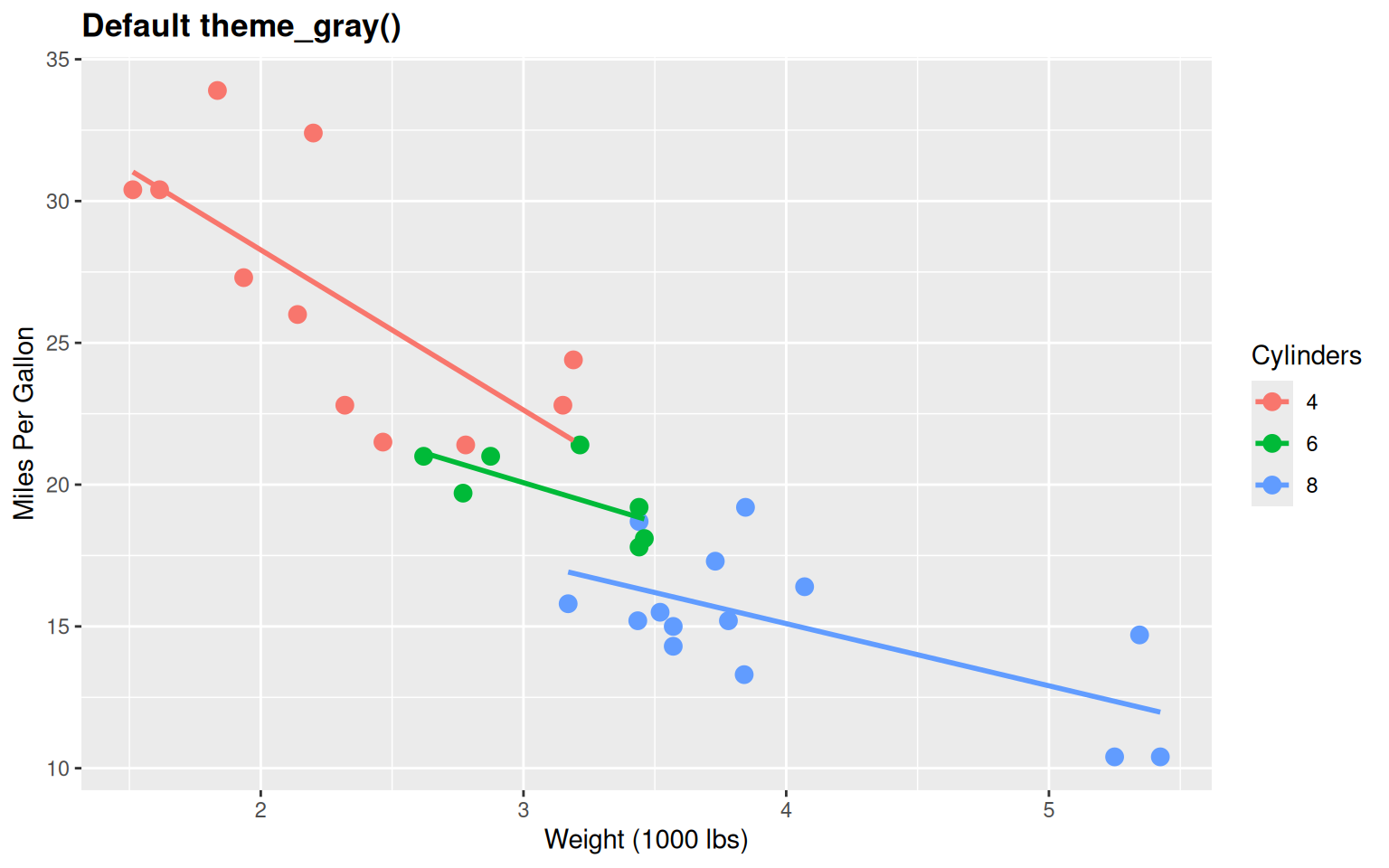

Problems:

• Gray background (wastes ink, unprofessional)
• Too much “chart junk”
• Not publication-ready

5.3 Built-in Theme: theme_bw()

p <- ggplot(mtcars, aes(wt, mpg, color = factor(cyl))) +
  geom_point(size = 3) +
  geom_smooth(method = "lm", se = FALSE) +
  labs(title = "theme_bw() - White background, black border",
       x = "Weight (1000 lbs)",
       y = "Miles Per Gallon",
       color = "Cylinders") +
  theme_bw() +
  theme(plot.title = element_text(face = "bold"))

`geom_smooth()` using formula = 'y ~ x'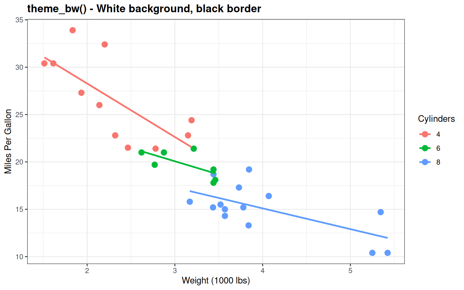

Good for publications - Clean with reference gridlines

5.4 Built-in Theme: theme_classic()

p <- ggplot(mtcars, aes(wt, mpg, color = factor(cyl))) +
  geom_point(size = 3) +
  geom_smooth(method = "lm", se = FALSE) +
  labs(title = "theme_classic() - No gridlines, clean axes",
       x = "Weight (1000 lbs)",
       y = "Miles Per Gallon",
       color = "Cylinders") +
  theme_classic() +
  theme(plot.title = element_text(face = "bold"))

`geom_smooth()` using formula = 'y ~ x'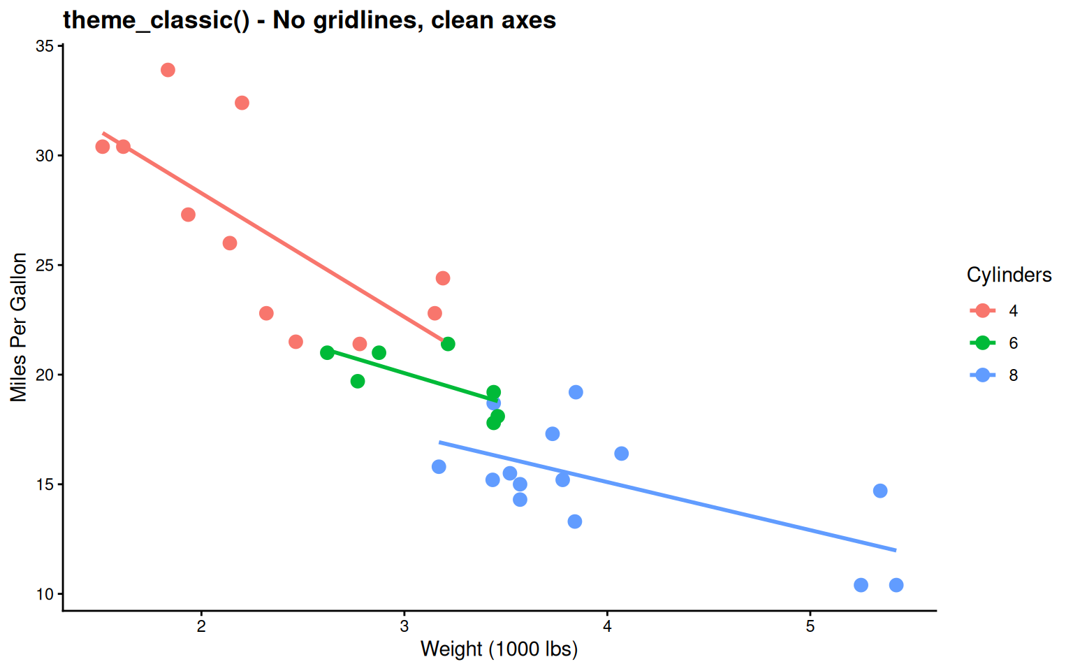

Very minimal - Traditional journal style

5.5 Built-in Theme: theme_minimal()

p <- ggplot(mtcars, aes(wt, mpg, color = factor(cyl))) +
  geom_point(size = 3) +
  geom_smooth(method = "lm", se = FALSE) +
  labs(title = "theme_minimal() - Subtle gridlines, modern",
       x = "Weight (1000 lbs)",
       y = "Miles Per Gallon",
       color = "Cylinders") +
  theme_minimal() +
  theme(plot.title = element_text(face = "bold"))

`geom_smooth()` using formula = 'y ~ x'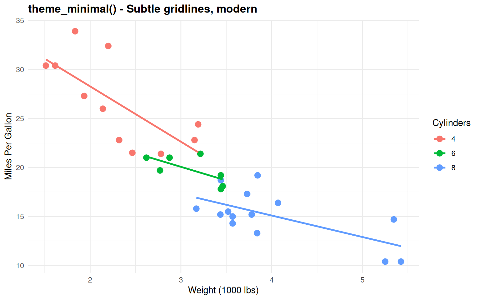

Good balance - Clean with subtle reference lines

5.6 Built-in Theme: theme_void()

p <- ggplot(mtcars, aes(wt, mpg, color = factor(cyl))) +
  geom_point(size = 3) +
  labs(title = "theme_void() - Blank canvas") +
  theme_void() +
  theme(plot.title = element_text(face = "bold", hjust = 0.5),
        legend.position = "right")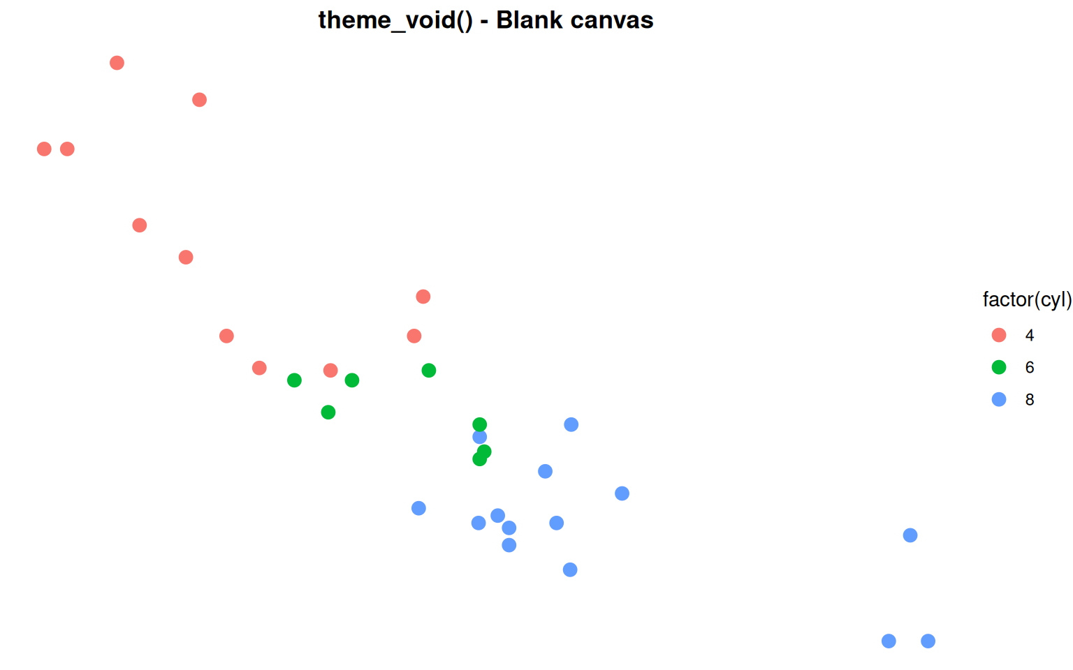

For custom designs - Maps, minimalist graphics

5.7 Side-by-Side Comparison

`geom_smooth()` using formula = 'y ~ x'
`geom_smooth()` using formula = 'y ~ x'
`geom_smooth()` using formula = 'y ~ x'
`geom_smooth()` using formula = 'y ~ x'
`geom_smooth()` using formula = 'y ~ x'
`geom_smooth()` using formula = 'y ~ x'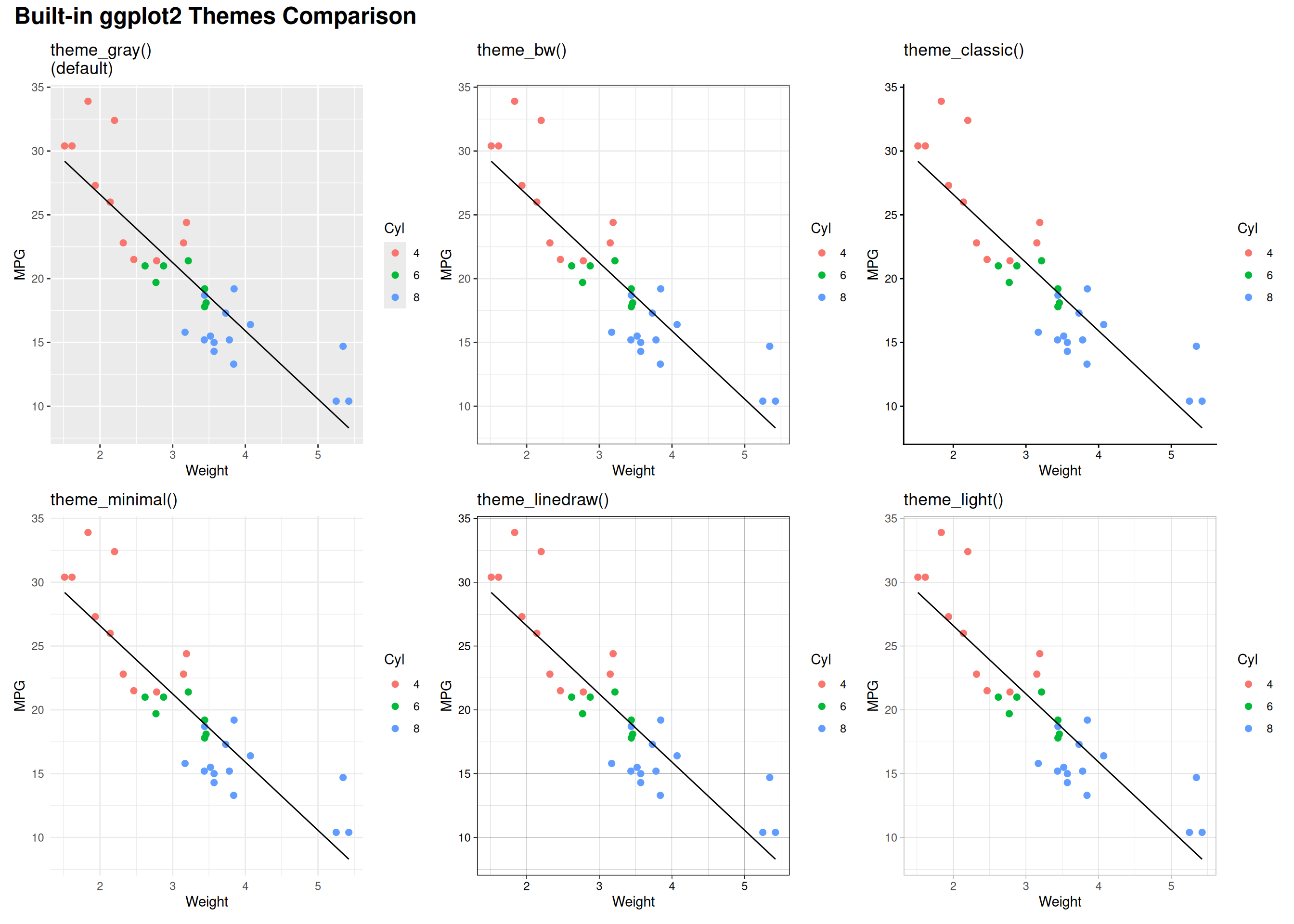

5.8 Publication Package: ggpubr

# ggpubr - publication-ready themes and statistical annotations
# install.packages("ggpubr")

ggplot(mtcars, aes(x = factor(cyl), y = mpg)) +
  geom_boxplot(aes(fill = factor(cyl)), alpha = 0.7) +
  geom_jitter(width = 0.2, alpha = 0.5) +
  labs(title = "ggpubr - Publication ready with stats",
       x = "Cylinders",
       y = "Miles Per Gallon") +
  theme_pubr() +
  theme(legend.position = "none",
        plot.title = element_text(face = "bold")) +
  scale_fill_brewer(palette = "Set2")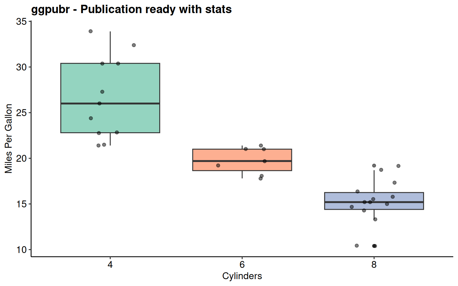

ggpubr Package

Publication-ready themes + statistical annotations

• theme_pubr() - Clean publication theme
• theme_pubclean() - Even more minimal
• stat_regline_equation() - Automatic regression equations
• stat_cor() - Correlation statistics
• stat_compare_means() - p-values and significance brackets

5.9 ggpubr: Adding Regression Equations

library(ggpubr)

p <- ggplot(mtcars, aes(x = wt, y = mpg)) +
  geom_point(size = 3, color = "steelblue") +
  geom_smooth(method = "lm", se = TRUE,
              color = "darkred", formula = y ~ x) +

      stat_regline_equation(
      aes(label = after_stat(eq.label)),
      formula = y ~ x,
      label.x.npc = 0.95,  # 95% to the right (relative)
      label.y.npc = 0.95,  # 95% to the top (relative)
      hjust = 1            # right-align text
    ) +
    stat_cor(
      aes(label = paste(after_stat(rr.label), after_stat(p.label), sep = "~~~~")),
      label.x.npc = 0.95, label.y.npc = 0.88, hjust = 1
    ) +
  
  labs(title = "Linear Regression with Equation",
       x = "Weight (1000 lbs)",
       y = "Miles Per Gallon") +
  theme_pubr()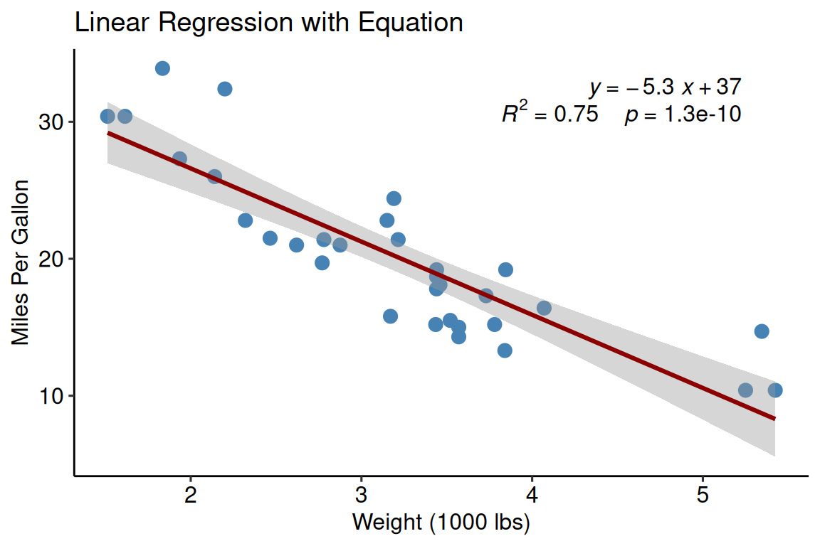

Key function: stat_regline_equation()

• Automatically calculates and displays equation
• Shows R² value
• Customizable position and formatting
• Works with facets

5.10 ggpubr: Pairwise Comparisons

# Automatically generate all pairwise comparisons
dose_levels <- levels(factor(ToothGrowth$dose))
my_comparisons <- combn(dose_levels, 2, simplify = FALSE)

p <- ggboxplot(ToothGrowth,
               x = "dose", y = "len", color = "dose", palette = "jco") +
  stat_compare_means(
                      comparisons = my_comparisons,
                      method = "t.test",
                      p.adjust.method = "BH"  # Benjamini-Hochberg (FDR) correction
                    ) +
  stat_compare_means(
                      method = "anova",
                      label.y = 50
                    ) +
  labs(title = "Pairwise Comparisons with Multiple Testing Correction",
       x = "Dose (mg/day)",
       y = "Tooth Length")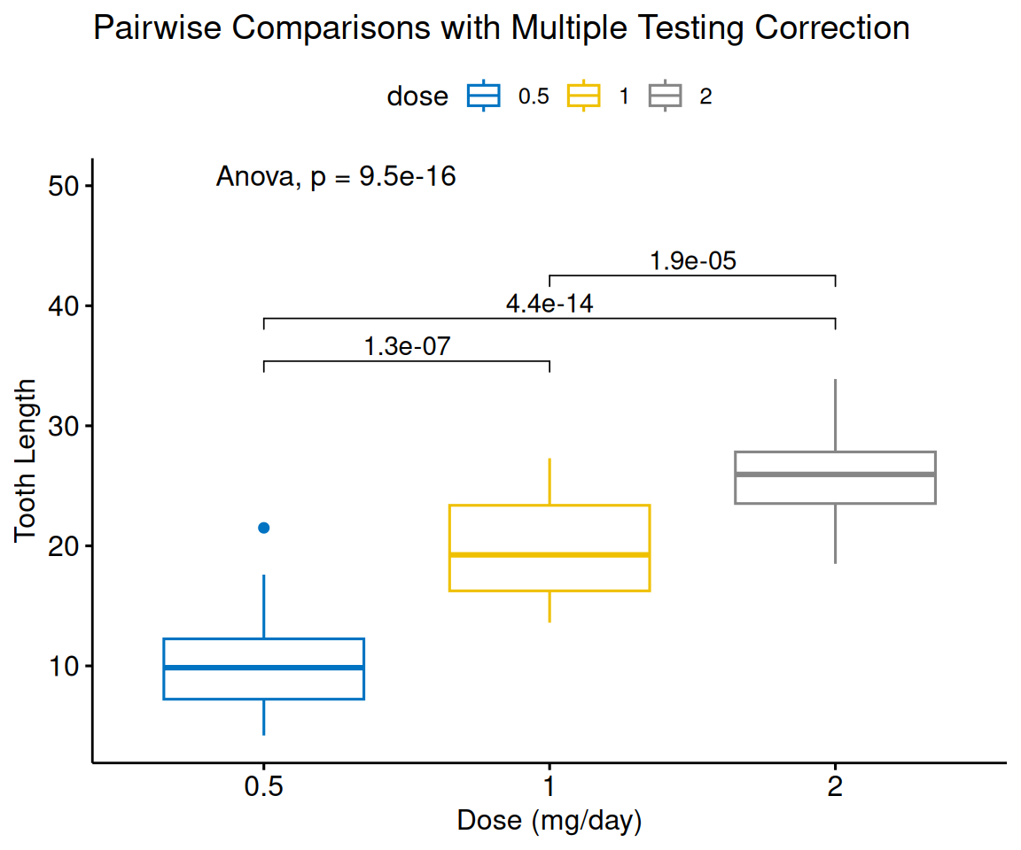

• combn(levels, 2) generates all pairs automatically
• method = "t.test" for pairwise tests (or method = "tukey_hsd" for Tukey’s HSD)
• p.adjust.method = "BH" for multiple testing correction (“holm”, “bonferroni”, “hochberg”, “BY”, “fdr”)
• method = "anova" for overall test
• Automatic significance brackets

5.11 Modern Typography: hrbrthemes

ggplot(mtcars, aes(wt, mpg, color = factor(cyl))) +
  geom_point(size = 3) +
  geom_smooth(method = "lm", se = FALSE, formula = y ~ x) +
  facet_wrap(~gear, labeller = label_both) +
  labs(title = "hrbrthemes::theme_ipsum() - Modern typography",
       subtitle = "Clean, professional, with excellent fonts and facets",
       x = "Weight (1000 lbs)",
       y = "Miles Per Gallon",
       color = "Cylinders") +
  theme_ipsum() +
  scale_color_ipsum()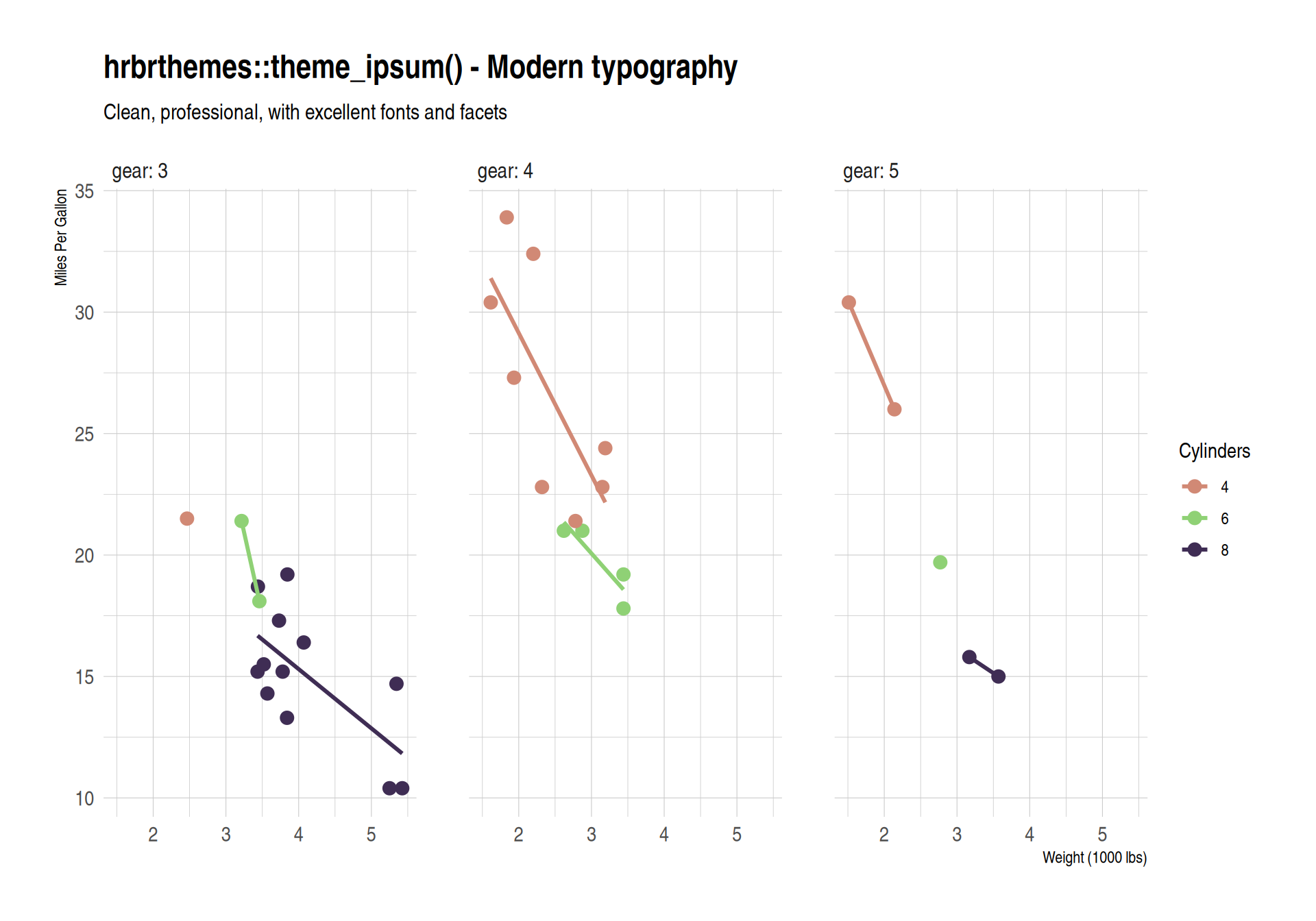

hrbrthemes Package

Modern professional typography

• Uses high-quality fonts (requires font installation)
• theme_ipsum() - Modern, clean, professional
• theme_ipsum_rc() - Roboto Condensed font
• Excellent for presentations and reports
• Works beautifully with facets
• May require: extrafont::font_import()

5.12 Specialized Themes: ggthemes

Warning: The `size` argument of `element_line()` is deprecated as of ggplot2 3.4.0.
ℹ Please use the `linewidth` argument instead.
ℹ The deprecated feature was likely used in the ggthemes package.
  Please report the issue at <https://github.com/jrnold/ggthemes/issues>.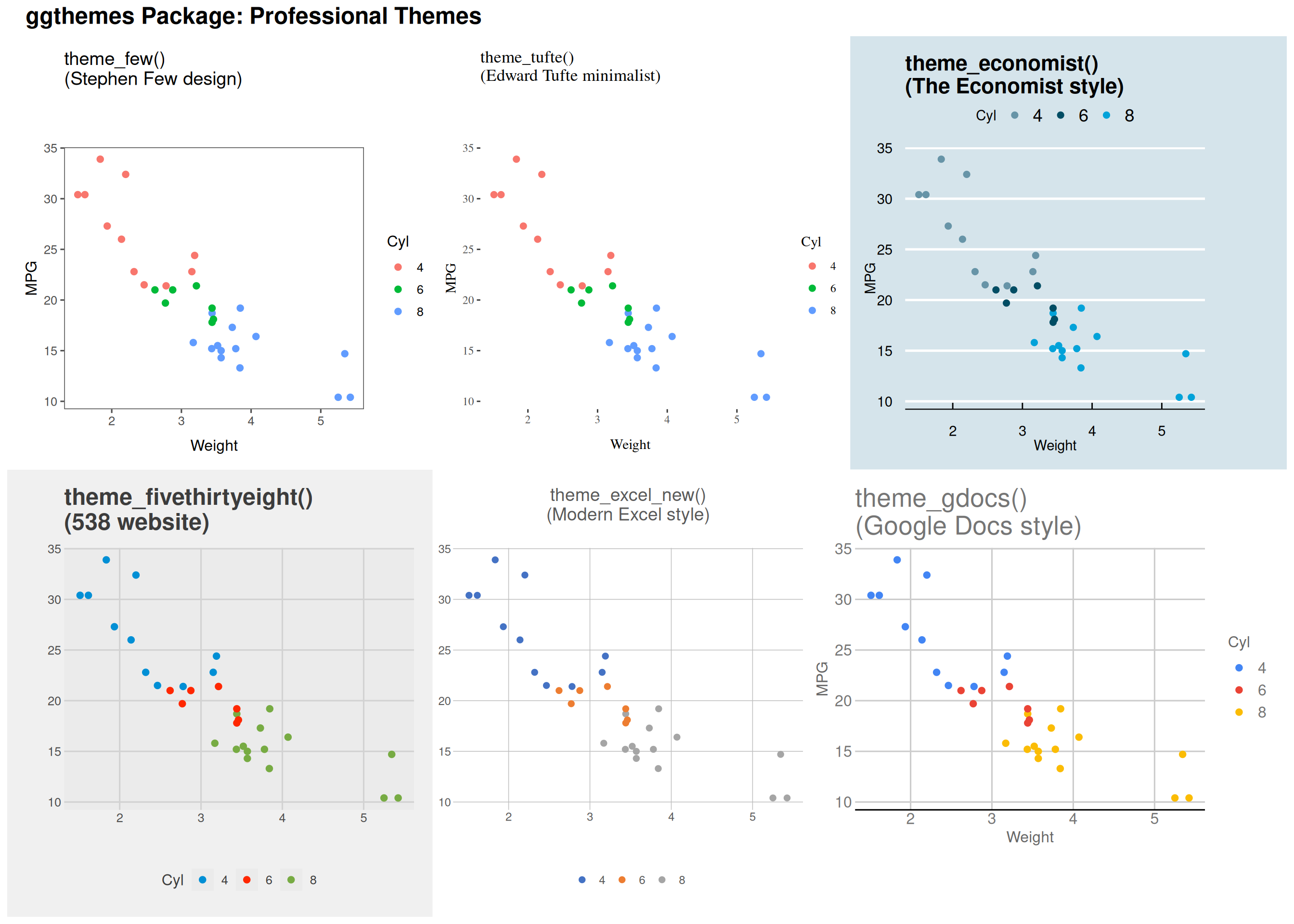

5.13 Setting Global Theme

Set once, apply to all plots:

# At top of script
theme_set(theme_bw(base_size = 12))

# Now all plots use theme_bw
# automatically
p1 <- ggplot(mtcars, aes(wt, mpg)) +
  geom_point() +
  labs(title = "Plot 1")

p2 <- ggplot(iris, aes(Sepal.Length, Sepal.Width)) +
  geom_point(aes(color = Species)) +
  labs(title = "Plot 2")

p3 <- ggplot(faithful, aes(eruptions)) +
  geom_histogram(bins = 30, fill = "steelblue") +
  labs(title = "Plot 3")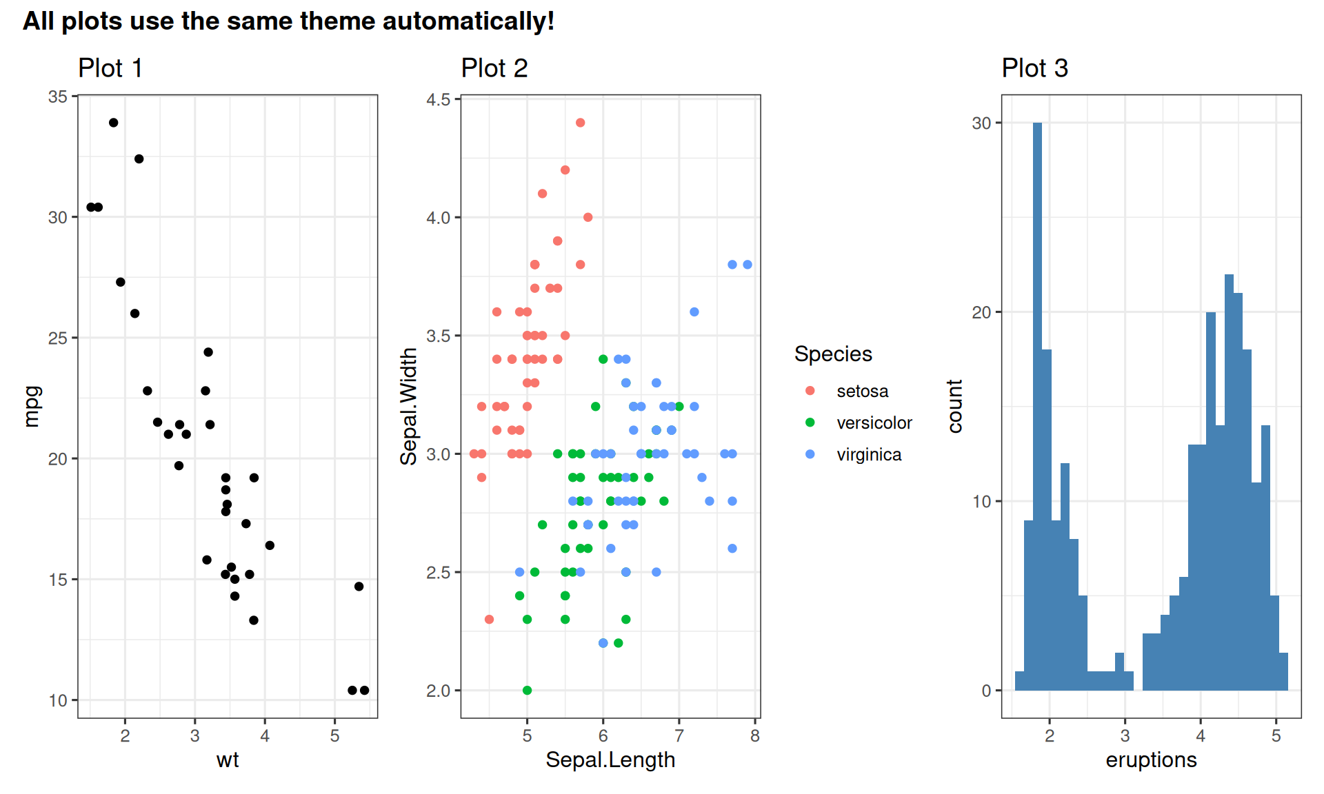

5.14 Font Considerations

# Check available fonts
# library(extrafont)
font_import()  # First time only (takes a while)
fonts()        # List available fonts

# Use in theme
theme_classic(base_family = "Arial") +
  theme(
    plot.title = element_text(family = "Arial", face = "bold"),
    axis.title = element_text(family = "Arial")
  )

Font Preferences by Journal

Many journals prefer specific fonts:

• Arial - Most common, widely accepted
• Helvetica - Classic choice
• Times New Roman - Traditional journals
• Calibri - Modern alternative

Check journal author guidelines!

5.15 Theme Elements You Can Customize

p <- ggplot(mtcars, aes(x = factor(cyl), y = mpg, fill = factor(cyl))) +
  geom_boxplot(alpha = 0.7) +
  facet_wrap(~gear, labeller = label_both) +
  labs(title = "Customized Theme Elements",
       x = "Cylinders",
       y = "Miles Per Gallon",
       fill = "Cylinders") +
  theme_minimal() +
  theme(
    # Axis elements
    axis.title = element_text(size = 12, face = "bold", color = "navy"),
    axis.text = element_text(size = 10, color = "gray30"),
    # Legend
    legend.position = "bottom",
    legend.title = element_text(face = "bold"),
    legend.background = element_rect(fill = "gray95", color = "gray50"),
    # Panel
    panel.grid.major = element_line(color = "gray80", linewidth = 0.3),
    panel.grid.minor = element_blank(),
    panel.background = element_rect(fill = "white"),
    # Facet strips
    strip.background = element_rect(fill = "steelblue", color = "navy"),
    strip.text = element_text(color = "white", face = "bold", size = 11),
    # Plot
    plot.title = element_text(size = 16, face = "bold", hjust = 0.5),
    plot.background = element_rect(fill = "white", color = NA)
  ) +
  scale_fill_brewer(palette = "Set2")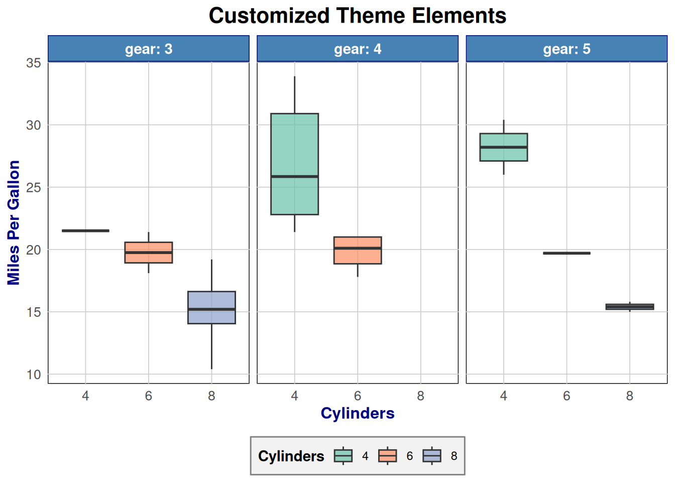

Customizable elements:

• axis.title, axis.text - Axis labels
• legend.position - “top”, “bottom”, “left”, “right”, “none”
• panel.grid - Gridlines
• plot.background, panel.background - Backgrounds
• strip.background, strip.text - Facet labels

5.16 Recommendations

Best Practices

1. Never use default theme_gray() for publications
   • Gray background wastes ink and looks unprofessional
2. Set global theme at start of script for consistency
   • theme_set(theme_classic()) applies to all subsequent plots
3. Match journal style - check published figures
   • Look at recent issues of your target journal
   • Note font choices, gridline presence, color schemes
4. Keep it simple - less chart junk = better
   • Remove unnecessary gridlines
   • Minimize non-data ink
5. Use publication packages for multi-panel figures
   • patchwork for intuitive combining syntax
   • ggpubr::ggarrange() for automatic labeling

5.17 Summary

Key Takeaways

1. Never use theme_gray() for publications - gray background wastes ink
2. Best built-in themes:
   • theme_classic() - clean, no gridlines (recommended for most cases)
   • theme_bw() - white background with gridlines
   • theme_minimal() - minimal gridlines, modern look
3. Set global theme: theme_set(theme_classic()) for consistency across all plots
4. Publication-ready packages:
   • hrbrthemes - modern, professional themes
   • ggthemes - journal-specific themes (e.g., theme_economist())
5. Multi-panel combining:
   • patchwork: intuitive + and / syntax
   • ggpubr::ggarrange(): automatic panel labeling (A, B, C)
6. Match your journal - check published figures for style guidance
7. Consistency is key - use the same theme throughout your manuscript

5.18 Exercises

Try It Yourself

1. Create a plot and compare all built-in themes:

   p <- ggplot(mtcars, aes(mpg, hp)) + geom_point()
   p + theme_gray()      # default
   p + theme_classic()   # recommended
   p + theme_bw()
   p + theme_minimal()
   p + theme_void()

2. Set a global theme and create 3 different plots - notice they all inherit the theme

3. Install hrbrthemes and try theme_ipsum()

4. Combine 4 plots using patchwork:

   (p1 + p2) / (p3 + p4) + plot_annotation(tag_levels = 'A')

5. Look at 3 recent papers in your target journal - which theme do they use?

5.19 Further Reading

• ggplot2 themes gallery - all built-in themes
• hrbrthemes package - modern themes with proper fonts
• patchwork guide - comprehensive combining tutorial
• ggthemes package - journal-specific themes
• Wilke (2019) - Chapter 22 on choosing themes