library(patchwork)

p1 | p2 | p3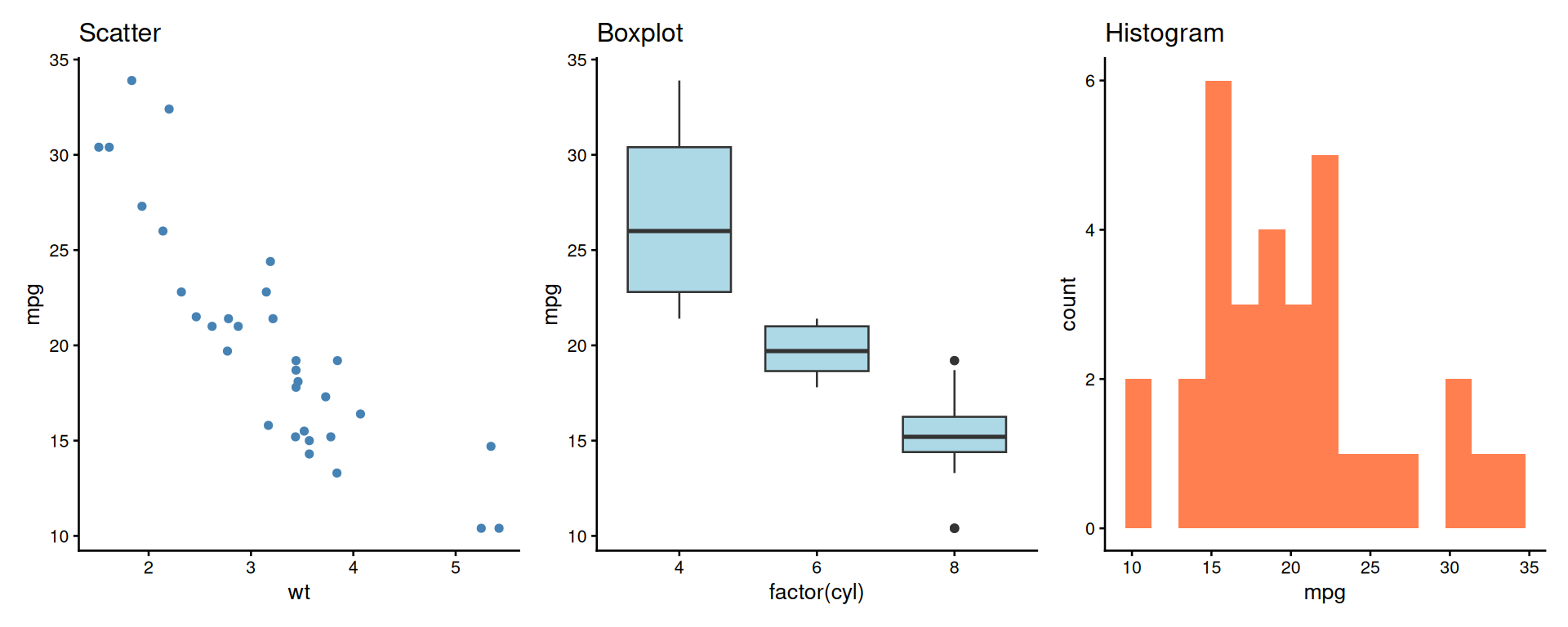
While everything should ideally be done in code for reproducibility, sometimes you need to edit exported figures manually—for example, to combine plots with photographs, add custom annotations, or achieve pixel-perfect alignment for publication. This chapter shows you the right tools and workflow for post-export editing while maintaining as much reproducibility as possible.
By the end of this chapter, you will:
Legitimate uses:
Inkscape
Other options:
DO NOT use Photoshop, GIMP, or other raster editors for plots!
Keep it vector! Use Inkscape, Illustrator, or PowerPoint with SVG input and PDF output.
Opening PDFs/SVGs:
Useful tools:
Tips:
Handling Missing Fonts:
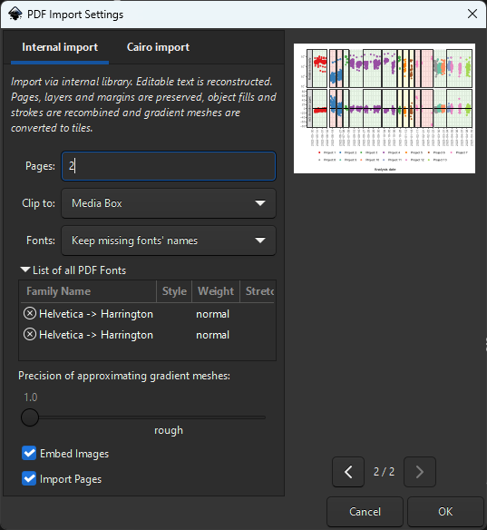
Keep the font names! Don’t substitute - preserves original font info and prevents text reflow issues
The Page Tool approach:
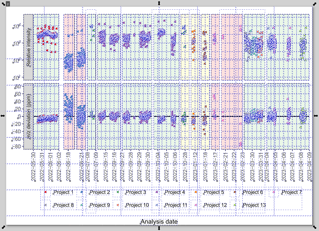
R exports contain many invisible/empty objects that prevent proper cropping!
The frustrating whack-a-mole:
Why clipping doesn’t work:
Original R output

After editing in Inkscape

Changes made:
A better alternative to manual composition!
library(patchwork)
p1 | p2 | p3
p1 / p2 / p3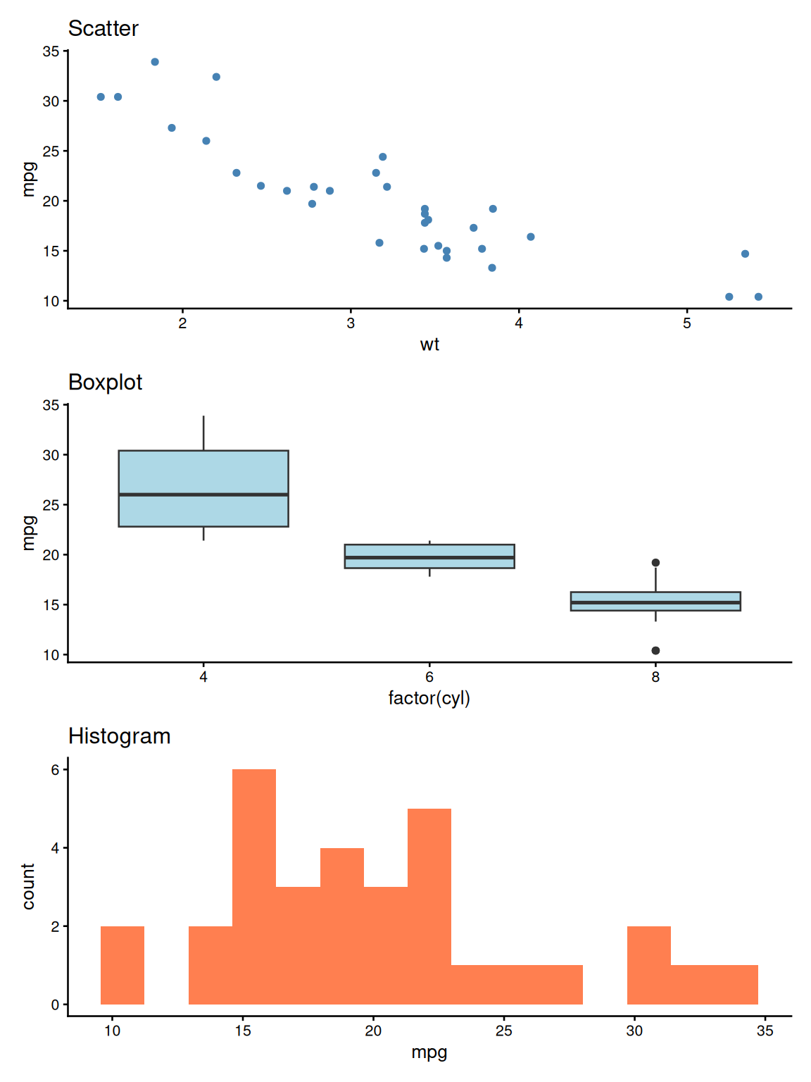
(p1 | p2) / (p3 | p4)`geom_smooth()` using formula = 'y ~ x'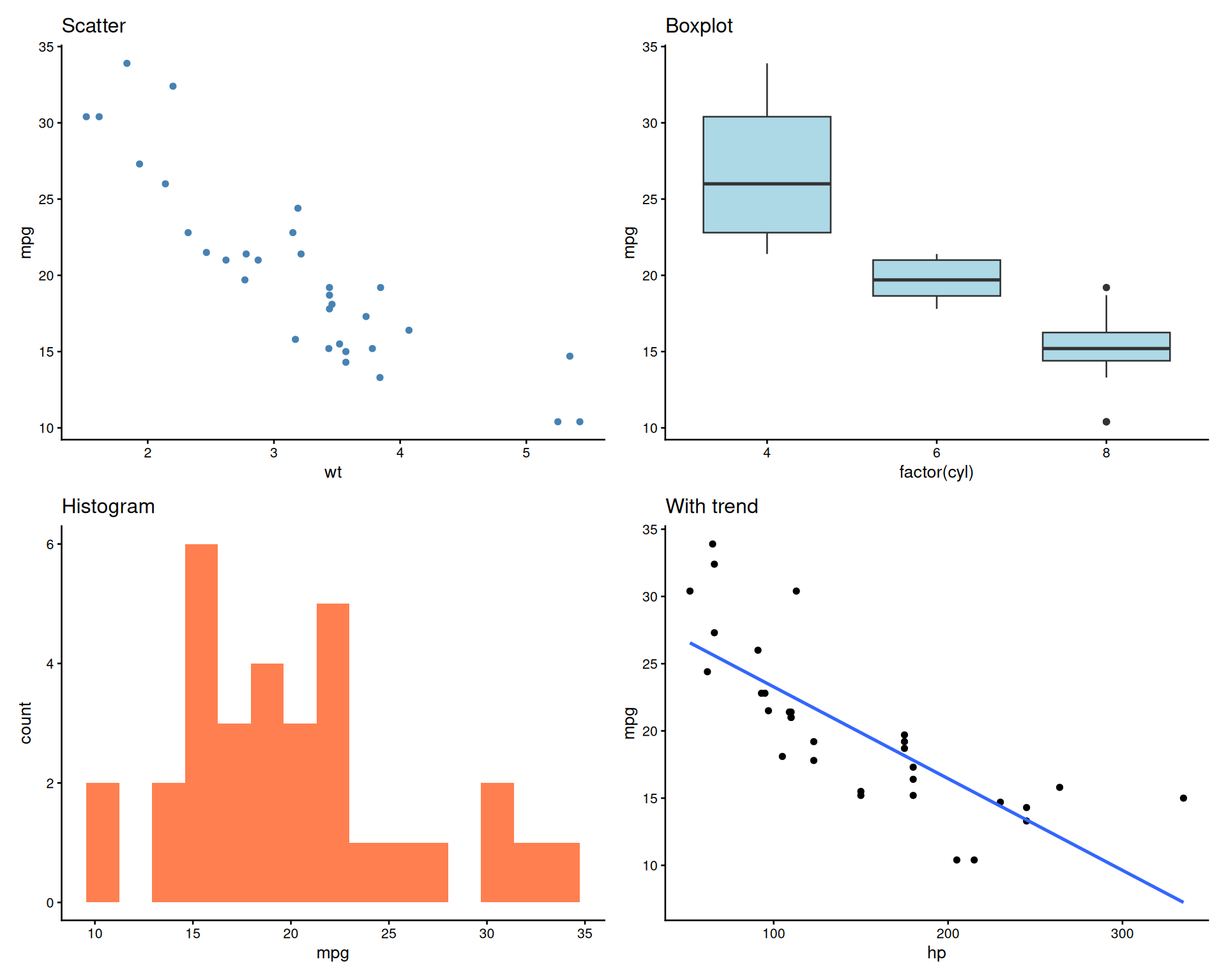
(p1 | p2) / (p3 | p4) +
  plot_annotation(tag_levels = 'A')
`geom_smooth()` using formula = 'y ~ x'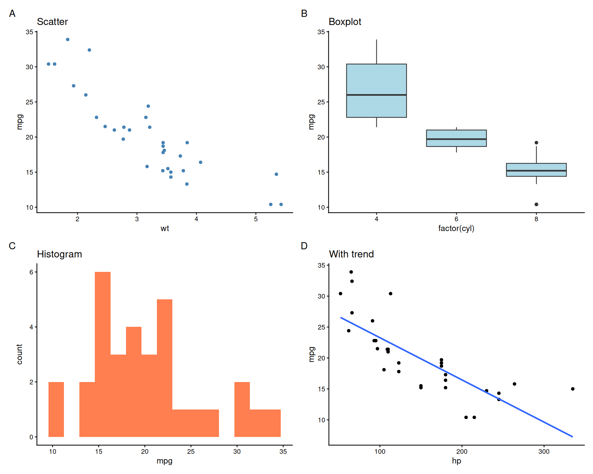
(p1 | p2) / (p3 | p4) +
  plot_annotation(
    tag_levels = 'A',
    tag_prefix = '(',
    tag_suffix = ')'
  ) &
  theme(plot.tag = element_text(face = 'bold', size = 14))
`geom_smooth()` using formula = 'y ~ x'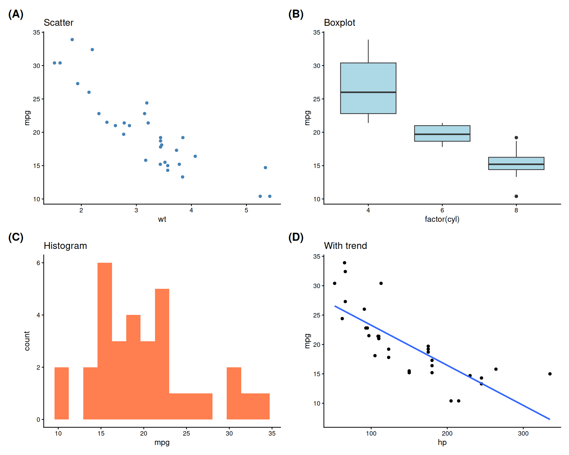
# First plot takes 2x width
p1 + p2 + p3 +
  plot_layout(widths = c(2, 1, 1)) +
  plot_annotation(tag_levels = 'A')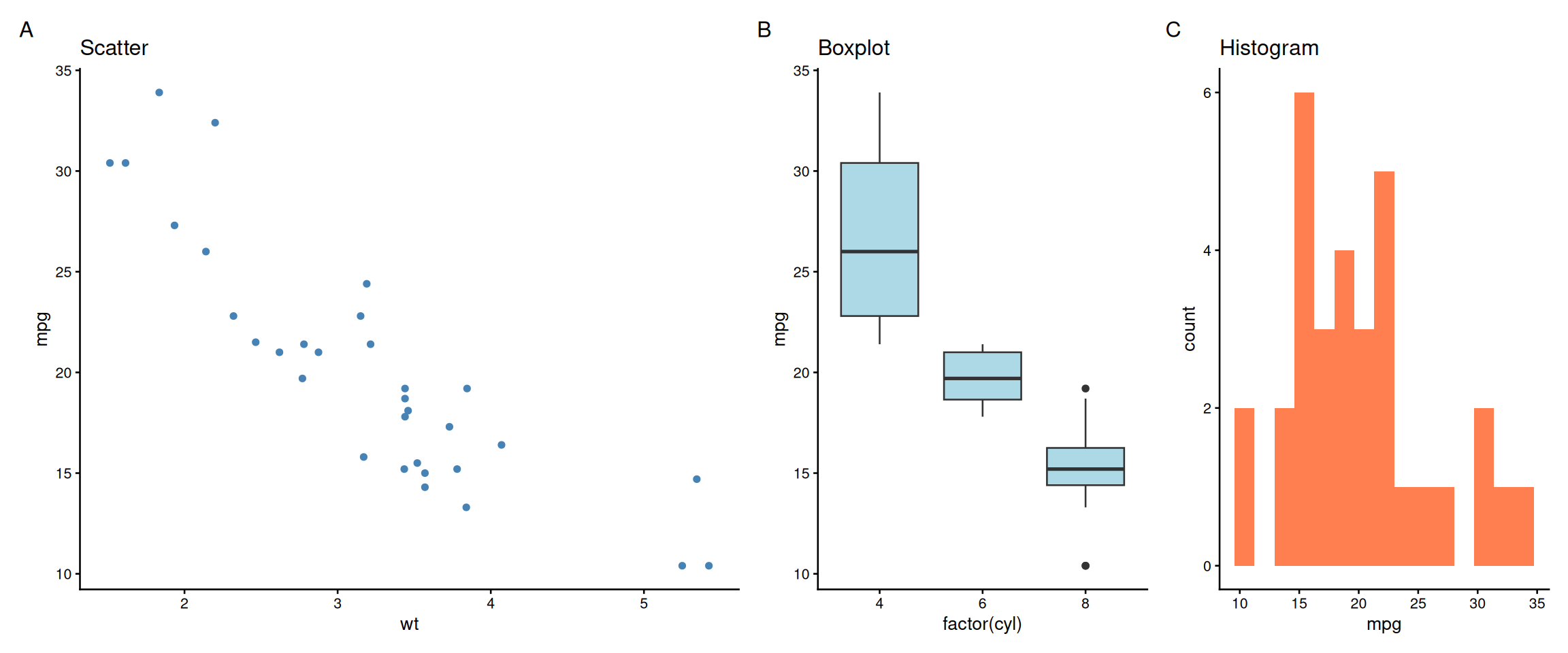
# Large plot on left, two stacked on right
p1 | (p2 / p3) +
  plot_annotation(tag_levels = 'A')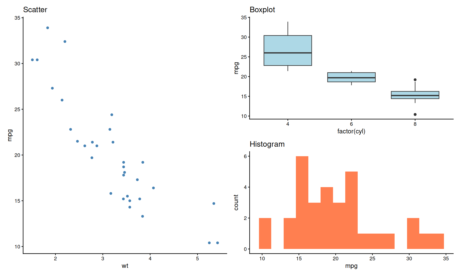
# Create plots with same color mapping
pa <- ggplot(mtcars, aes(wt, mpg, color = factor(cyl))) +
  geom_point() + theme_classic(base_size = 10)
pb <- ggplot(mtcars, aes(hp, mpg, color = factor(cyl))) +
  geom_point() + theme_classic(base_size = 10)

pa + pb +
  plot_layout(guides = 'collect') +
  plot_annotation(tag_levels = 'A')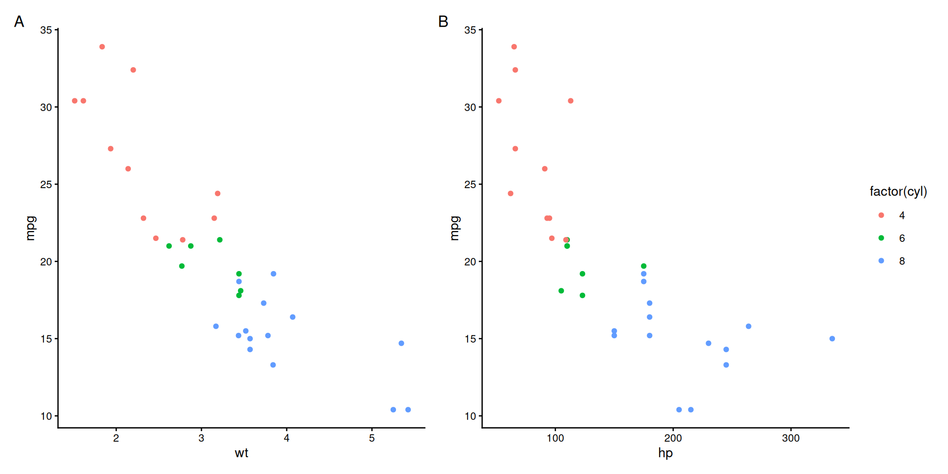
# Share y-axes for side-by-side plots
(p1 | p2) + plot_layout(axes = "collect_y")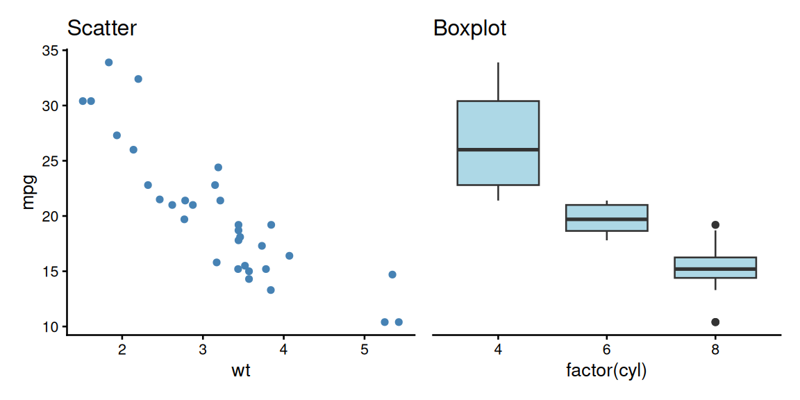
collect_x: Remove duplicate x-axes when plots are stacked vertically (same x-scale)collect_y: Remove duplicate y-axes when plots are side-by-side (same y-scale)collect: Remove both x and y axes (same scales in both directions)# Complex: collect within groups first
((p1 | p2) + plot_layout(axes = "collect_y")) /
(p3 | p4)`geom_smooth()` using formula = 'y ~ x'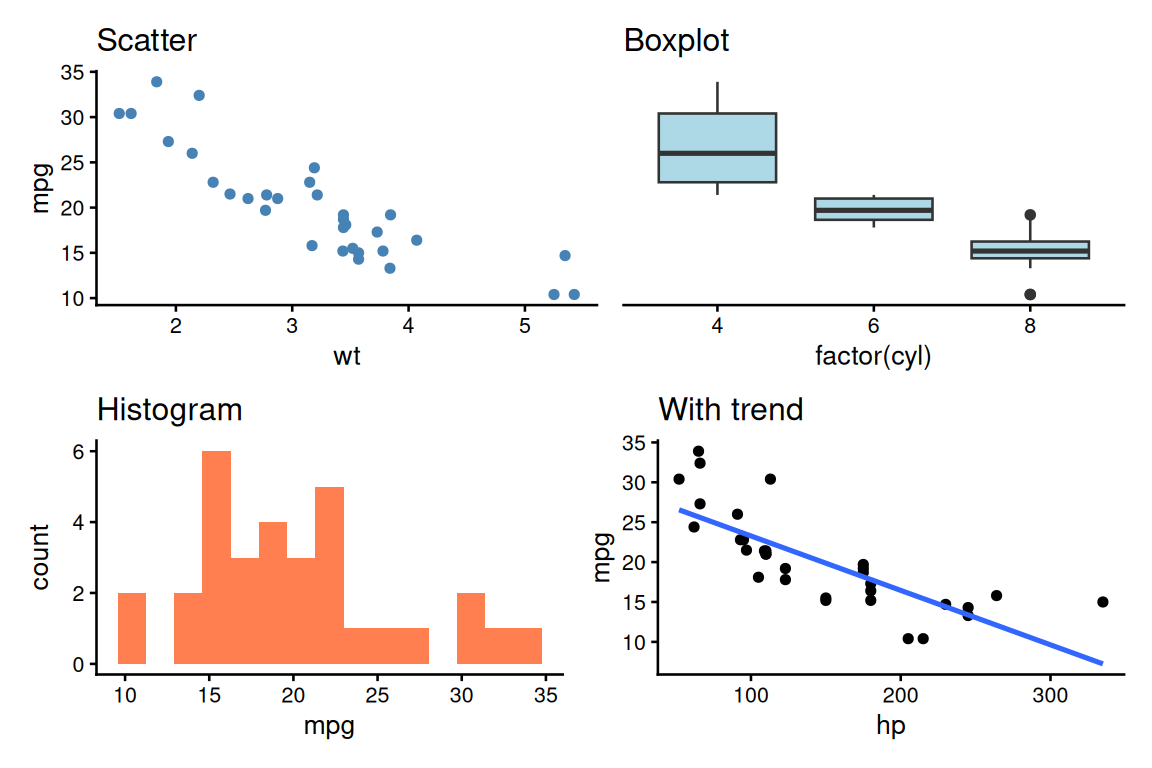
Benefits:
# Create combined figure
combined <- (p1 | p2) / (p3 | p4) +
  plot_annotation(tag_levels = 'A')

# Save as vector (recommended)
ggsave("figure1.svg", combined, width = 10, height = 8)
ggsave("figure1.pdf", combined, width = 10, height = 8)

# Save as high-res raster if needed
ggsave("figure1.png", combined, width = 10, height = 8, dpi = 300)patchwork (in R)
✅ Fully reproducible
✅ Easy to update
✅ Automatic alignment
✅ Consistent styling
✅ Version controlled
⚠️ Less layout flexibility
Use patchwork when:
Inkscape (manual editing)
✅ Pixel-perfect control
✅ Mix with non-R content
✅ Complex annotations
❌ Not reproducible
❌ Manual re-editing
❌ Easy to break
Use Inkscape when:
patchwork or cowplot for combining plotsggforce for annotations and custom shapesgrid for precise layout controlpatchwork in R - which was easier?