# Create data with logical categories
category_df <- data.frame(
  category = c("Low", "Medium", "High", "Very High", "Low", "High"),
  value = c(10, 20, 15, 30, 12, 25)
)

# R defaults to alphabetical!
p1 <- ggplot(category_df, aes(x = category, y = value)) +
  geom_col(fill = "coral") +
  theme_classic(base_size = 12) +
labs(title = "Alphabetical (Wrong!)")9 Factor Ordering
9.1 Introduction
R’s factor system is both powerful and treacherous. Alphabetical ordering makes categorical plots hard to read, and accidental conversion of numeric factors causes data corruption. This chapter teaches you how to control factor ordering and avoid common pitfalls.
Learning Objectives
By the end of this chapter, you will:
- Understand why alphabetical factor ordering is rarely useful
- Learn to reorder factors by frequency, by another variable, or manually
- Master the
forcatspackage for factor manipulation - Know how to properly convert factors to numeric without data loss
- Avoid the “numeric factor” trap (numbered categories vs. actual numbers)
- Create publication-ready plots with meaningful orderings
9.2 The Problem: Alphabetical Ordering
# Specify levels explicitly
category_df$category <- factor(category_df$category,
                       levels = c("Low", "Medium", "High", "Very High"))

# Now plots use logical order!
p2 <- ggplot(category_df, aes(x = category, y = value)) +
  geom_col(fill = "steelblue") +
  theme_classic(base_size = 12) +
  labs(title = "Logical Order (Correct!)")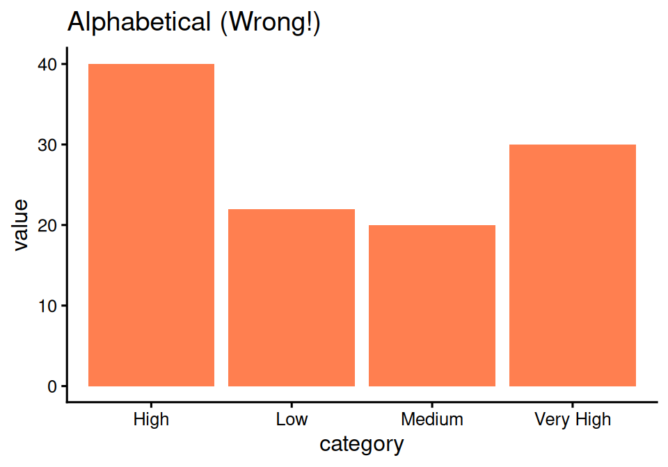
Random order makes no sense!
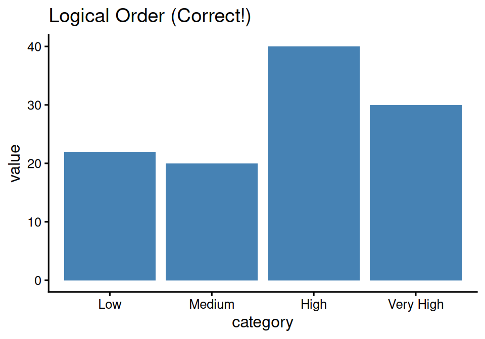
Much better - order makes sense!
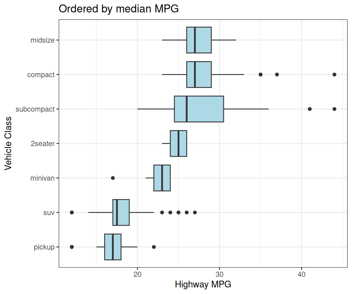
9.3 Solution: forcats Package
Part of tidyverse, designed for factor manipulation
library(forcats)

# Reorder car classes by median highway mpg
p <- mpg %>%
  ggplot(aes(x = fct_reorder(class, hwy, median),
             y = hwy)) +
  geom_boxplot(fill = "lightblue") +
  coord_flip() +
  labs(x = "Vehicle Class",
       y = "Highway MPG",
       title = "Ordered by median MPG")
Boxplots now ordered by median value!
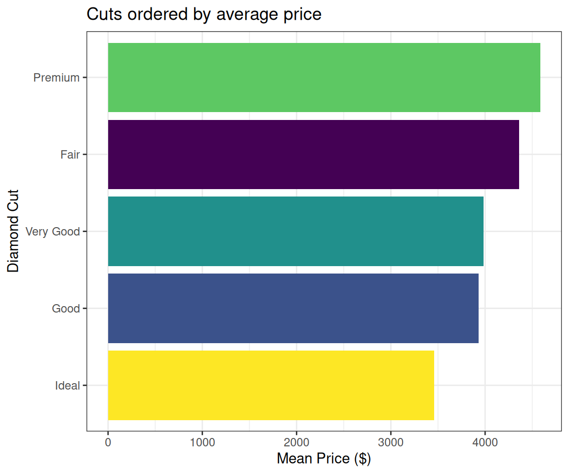
9.4 fct_reorder(): Order by Another Variable
# Order diamond cuts by mean price
p <- diamonds %>%
  group_by(cut) %>%
  summarise(mean_price = mean(price)) %>%
  ggplot(aes(x = fct_reorder(cut, mean_price),
             y = mean_price,
             fill = cut)) +
  geom_col(show.legend = FALSE) +
  coord_flip() +
  labs(x = "Diamond Cut",
       y = "Mean Price ($)",
       title = "Cuts ordered by average price")
Bars ordered by length!
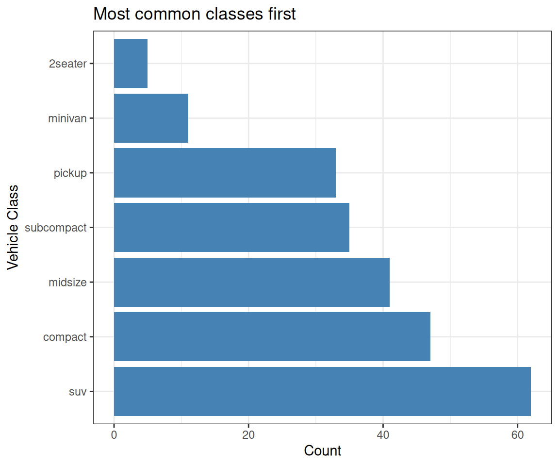
9.5 fct_infreq(): Order by Frequency
# Order by how common each vehicle class is
p <- ggplot(mpg,
            aes(x = fct_infreq(class))) +
  geom_bar(fill = "steelblue") +
  coord_flip() +
  labs(x = "Vehicle Class",
       y = "Count",
       title = "Most common classes first")
Most common category first!
Great for survey data
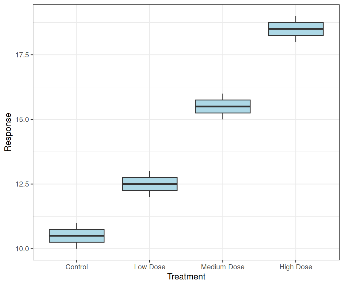
9.6 fct_inorder(): Order by Appearance
# Create data with specific order
treatment_data <- data.frame(
  treatment = c("Control", "Low Dose",
                "Medium Dose", "High Dose",
                "Control", "Low Dose",
                "Medium Dose", "High Dose"),
  response = c(10, 12, 15, 18,
               11, 13, 16, 19)
)

# Keep order as they appear in data
p <- ggplot(treatment_data,
       aes(x = fct_inorder(treatment),
           y = response)) +
  geom_boxplot(fill = "lightblue") +
  labs(x = "Treatment", y = "Response")
Preserves the order from your data!
9.7 Natural Sorting: var1, var2, …, var10
The problem with alphabetical sorting:
# Create data with numbered variables
var_data <- data.frame(
  variable = rep(c("var1", "var2", "var10", "var20"), each = 5),
  value = rnorm(20, mean = rep(c(10, 15, 20, 25), each = 5), sd = 2)
)

# Alphabetical order: var1, var10, var2, var20 (wrong!)
p <- ggplot(var_data, aes(x = variable, y = value)) +
  geom_boxplot(fill = "coral") +
  labs(title = "Alphabetical: var1, var10, var2, var20")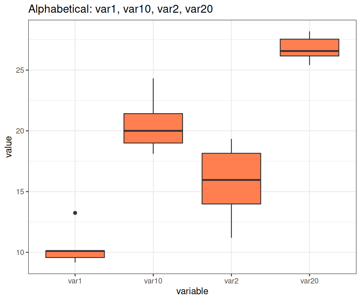
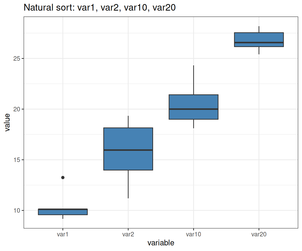
9.8 Natural Sorting: The Solution
# Use gtools::mixedsort() for natural/alphanumeric sorting
library(gtools)

var_data$variable <- factor(var_data$variable,
                            levels = mixedsort(unique(var_data$variable)))

# Natural order: var1, var2, var10, var20 (correct!)
p <- ggplot(var_data, aes(x = variable, y = value)) +
  geom_boxplot(fill = "steelblue") +
  labs(title = "Natural sort: var1, var2, var10, var20")
Note: forcats::fct_inseq() only works if factor levels are purely numeric strings (e.g., “1”, “2”, “10”), not mixed alphanumeric like “var1”, “var10”
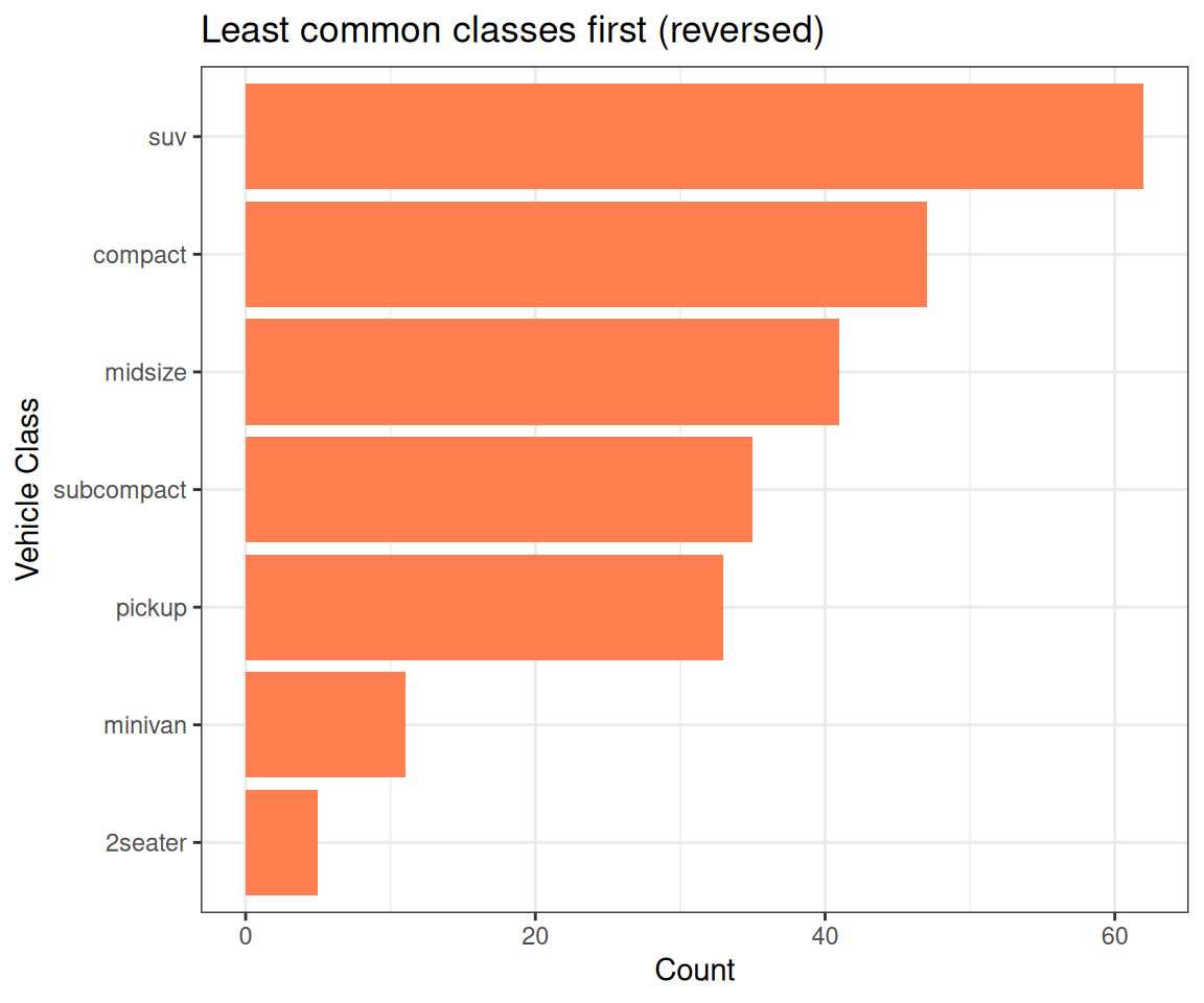
9.9 fct_rev(): Reverse Order
# Reverse the frequency order
p <- ggplot(mpg, aes(x = fct_rev(fct_infreq(class)))) +
  geom_bar(fill = "coral") +
  coord_flip() +
  labs(x = "Vehicle Class", y = "Count",
       title = "Least common classes first (reversed)")
Now least common first instead of most common!
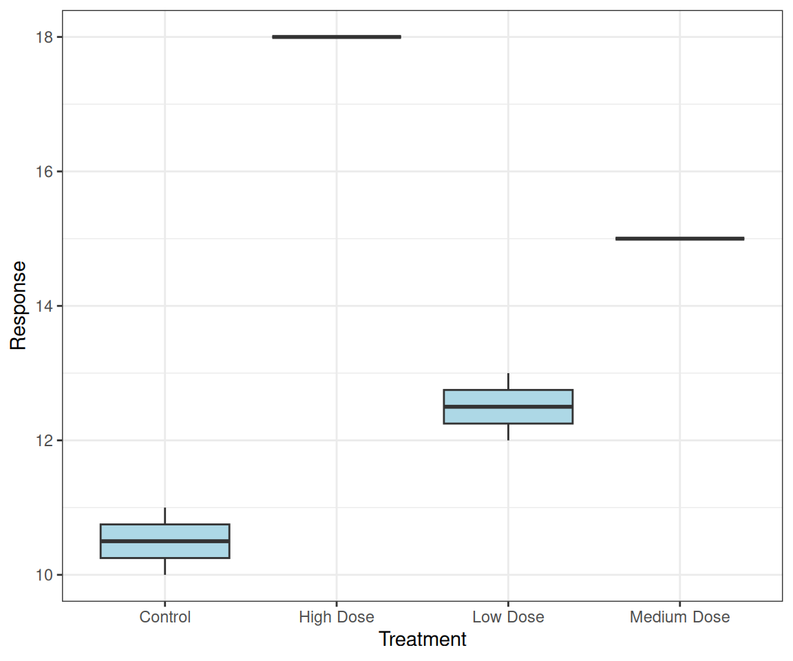
9.10 fct_relevel(): Move Specific Levels
# Move "Control" to front for treatment groups
treatment_data <- data.frame(
  treatment = c("Low Dose", "High Dose", "Control",
                "Medium Dose", "Low Dose", "Control"),
  response = c(12, 18, 10, 15, 13, 11)
)

p <- treatment_data %>%
  mutate(treatment = fct_relevel(treatment, "Control")) %>%
  ggplot(aes(treatment, response)) +
  geom_boxplot(fill = "lightblue") +
  labs(x = "Treatment", y = "Response")
Control always shown first
Common in experimental data!
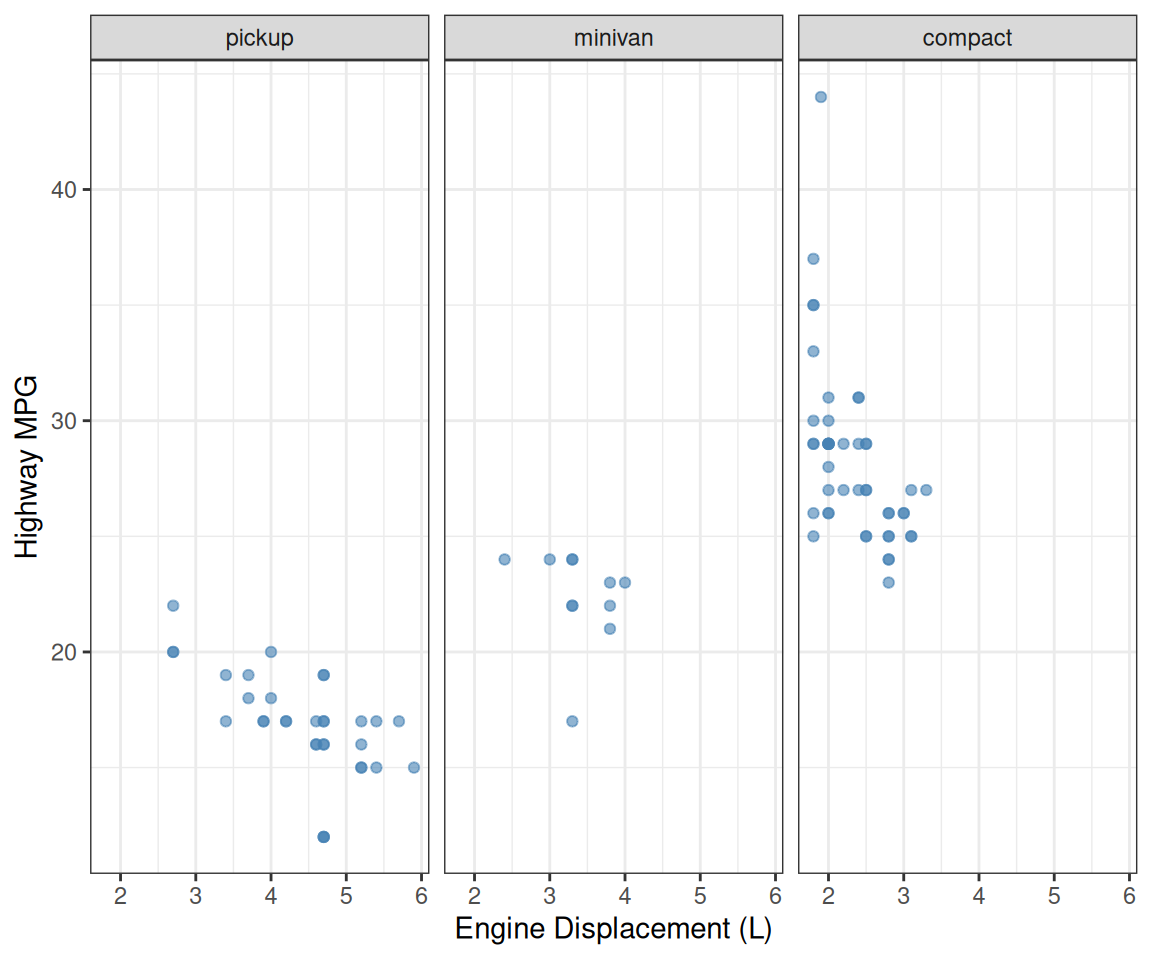
9.11 Facet Ordering
# Order facets by median highway mpg for each vehicle class
p <- mpg %>%
  filter(class %in% c("pickup", "minivan", "compact")) %>%
  mutate(class = fct_reorder(class, hwy, median)) %>%
  ggplot(aes(x = displ, y = hwy)) +
  geom_point(color = "steelblue", alpha = 0.6) +
  facet_wrap(~class) +
  labs(x = "Engine Displacement (L)", y = "Highway MPG")
Facet panels in meaningful order!
9.12 ⚠️ The Danger of Numeric Factors
Converting between factor and numeric can destroy your data!
# Original numeric data
doses <- c(10, 20, 50, 100, 200)
print(doses)
[1] 10 20 50 100 200# Convert to factor (common in data import!)
dose_factor <- factor(doses)
print(dose_factor)[1] 10 20 50 100 200
Levels: 10 20 50 100 200
# Looks fine, right? But look at the internal structure:
str(dose_factor)
Factor w/ 5 levels "10","20","50",..: 1 2 3 4 5levels(dose_factor)[1] "10" "20" "50" "100" "200"
# Try to convert back to numeric - WRONG!
as.numeric(dose_factor)
[1] 1 2 3 4 5# Correct way: convert via character
as.numeric(as.character(dose_factor))[1] 10 20 50 100 200
The danger: Many functions silently convert factors to integers!
9.13 ⚠️ Missing Levels: The Silent Data Corruption
Even worse: missing levels get renumbered!
  subject response
1       1       10
2       2       15
3       4       25
4       5       30
5       1       11
6       2       16
7       4       24
8       5       29
# Convert to factor (happens during import!)
subject_factor <- factor(subject)
str(subject_factor) Factor w/ 4 levels "1","2","4","5": 1 2 3 4 1 2 3 4Levels: “1” “2” “4” “5” - looks OK…
# Try to convert back - DATA CORRUPTION!
as.numeric(subject_factor)
[1] 1 2 3 4 1 2 3 4Returns: 1 2 3 4 1 2 3 4
Your subject 4 became 3!
Your subject 5 became 4!
This is catastrophic for analysis!
Your statistical models and plots will use the wrong subject numbers. Always use as.numeric(as.character(factor)) not as.numeric(factor).
Or better yet. NEVER use numbers for categorical data!
9.14 ⚠️ Numeric Factors After Reordering
dose_data <- tibble(
  dose = factor(c(0, 10, 50, 100, 200)),
  response = c(5, 25, 80, 70, 30)
) %>%
  mutate(dose_ordered =
         fct_reorder(dose, response))

dose_data
# A tibble: 5 × 3
dose response dose_ordered
<fct> <dbl> <fct>
1 0 5 0
2 10 25 10
3 50 80 50
4 100 70 100
5 200 30 200 # Try to use numerically - DISASTER!
dose_data <- dose_data %>%
mutate(
wrong = as.numeric(dose_ordered),
correct = as.numeric(as.character(dose_ordered))
)# A tibble: 5 × 5
dose response dose_ordered wrong correct
<fct> <dbl> <fct> <dbl> <dbl>
1 0 5 0 1 0
2 10 25 10 2 10
3 50 80 50 5 50
4 100 70 100 4 100
5 200 30 200 3 200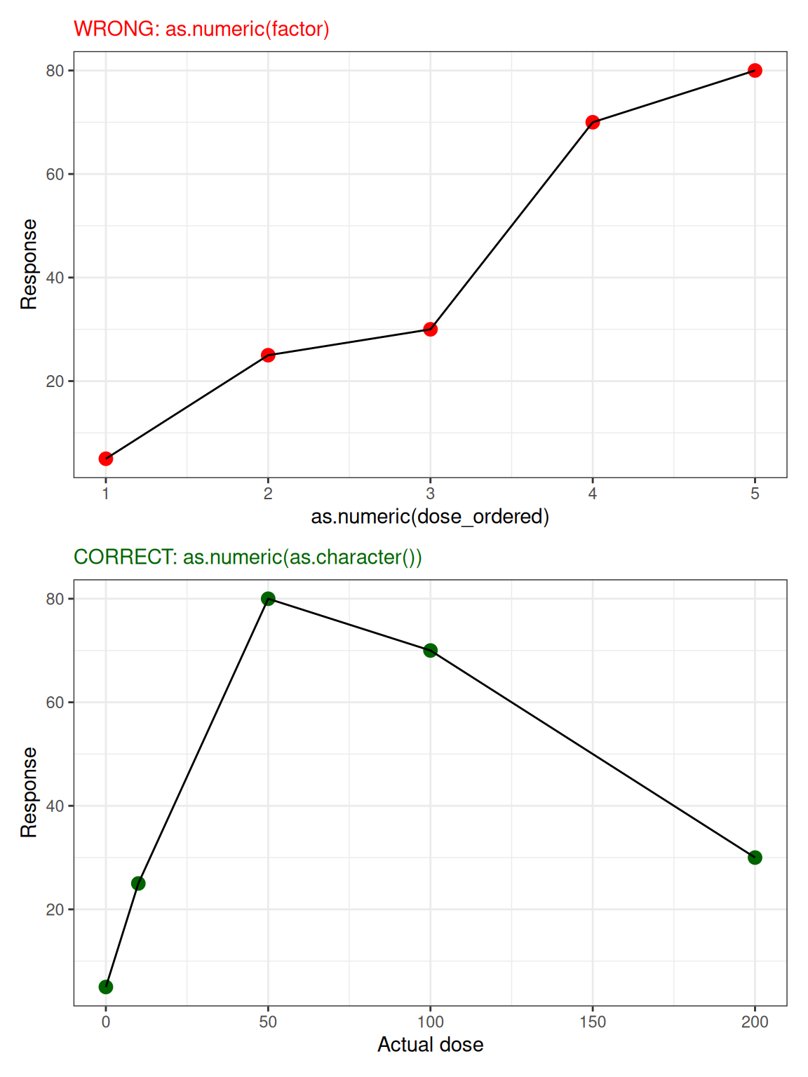
9.15 Recommendations: Avoid Numeric Factors
Best Practices
- Never store numeric values as factors unless they represent categories
- Prefix categorical numbers: Use “Group_1”, “Group_2” instead of “1”, “2”
- Check imported data: CSV imports often convert numbers to factors
- Use
readr::read_csv()instead ofread.csv()- better type detection and no implicit conversion to factors. - Always convert via character:
as.numeric(as.character(factor))notas.numeric(factor) - Check with
str()before analysis to verify data types
Bad: Numeric categories
# DON'T do this - ambiguous!
groups <- factor(c(1, 2, 4, 5))
str(groups)
Factor w/ 4 levels "1","2","4","5": 1 2 3 4# Are these numbers or categories?Good: Prefixed categories
# DO this - clearly categorical!
groups <- factor(c("Group_1", "Group_2",
                   "Group_4", "Group_5"))
str(groups)
Factor w/ 4 levels "Group_1","Group_2",..: 1 2 3 4# Obviously categories, safe!9.16 forcats Cheat Sheet
library(forcats)

fct_reorder(f, x, fun)   # Order by another variable
fct_infreq(f)            # Order by frequency
fct_inorder(f)           # Order by appearance in data
fct_inseq(f)             # Order by numeric value (if purely numeric)
fct_rev(f)               # Reverse current order
fct_relevel(f, "A", "B") # Move specific levels to front
fct_recode(f, new = "old") # Rename levels
fct_lump_n(f, n = 5)     # Keep top n, lump others as "Other"
fct_explicit_na(f)       # Make NA a visible level

# For natural sort (var1, var2, var10):
factor(x, levels = gtools::mixedsort(unique(x)))
9.17 Debugging Factor Issues
# Example: vehicle classes in mpg dataset
vehicle_class <- factor(mpg$class)

# Check level order
vehicle_class %>% levels()
[1] "2seater" "compact" "midsize" "minivan" "pickup"
[6] "subcompact" "suv" # See factor structure (shows integer encoding)
str(vehicle_class) Factor w/ 7 levels "2seater","compact",..: 2 2 2 2 2 2 2 2 2 2 ...# Check how many observations per level
table(vehicle_class)vehicle_class
2seater compact midsize minivan pickup subcompact suv
5 47 41 11 33 35 62 # Convert to character if needed for text operations
class_char <- as.character(vehicle_class)9.18 Key Takeaways & Best Practices
Remember
The Problem:
- R defaults to alphabetical factor ordering - usually wrong!
- Numeric factors are dangerous - converting destroys your data
- Missing levels get renumbered - group 4 becomes 3!
The Solutions:
- forcats package provides powerful ordering tools:
fct_reorder()orders by another variable (most useful!)fct_infreq()orders by frequencyfct_relevel()to put control/baseline firstfct_rev()to reverse order
- Manual levels for logical ordering (Low/Med/High, months, etc.)
- Prefix categorical numbers: “Group_1” not “1”
Always:
- Check factor order before plotting with
str()orlevels() - Convert via character:
as.numeric(as.character(f))notas.numeric(f) - Think about your reader - what order makes sense?
9.19 Summary
Key Takeaways
Alphabetical order is rarely useful - readers can’t interpret patterns
forcats package provides essential tools:
fct_reorder(category, value)- order by another variable (most common!)fct_infreq()- order by frequency (highest first)fct_rev()- reverse current orderfct_relevel(f, "Control")- move specific level first
Manual ordering for logical sequences:
factor(x, levels = c("Low", "Medium", "High"))
factor(month, levels = month.name)  # built-in constant
The numeric factor trap:
as.numeric(factor(c("1", "2", "10")))gives1, 2, 3(WRONG!)as.numeric(as.character(factor(c("1", "2", "10"))))gives1, 2, 10(correct)
Prefix numbered categories: Use “Group_1” not “1” to prevent accidental conversion
Always check:
str(data)andlevels(variable)before plottingThink about your reader: What ordering tells the story best?
9.20 Exercises
Try It Yourself
Create a dataset with unordered categories and fix the ordering:
df <- data.frame(
  treatment = c("High", "Low", "Medium", "High", "Low"),
  response = c(8.2, 3.1, 5.5, 9.1, 2.8)
)
# Fix: factor(treatment, levels = c("Low", "Medium", "High"))
Practice
fct_reorder():starwars %>% mutate(species = fct_reorder(species, height, .fun = median, na.rm = TRUE)) %>% ggplot(aes(height, species)) + geom_boxplot()Create a factor from numbers (“1”, “2”, “10”) and practice safe conversion
Compare plots with alphabetical vs. reordered factors - which is easier to read?
9.21 Further Reading
- forcats package documentation - comprehensive guide
- R for Data Science - Factors chapter - Hadley Wickham
- Factor ordering in ggplot2 - limits parameter
- The factor trap - common pitfalls