pdf("myplot.pdf", width = 7, height = 5)
  plot(x, y)
dev.off() # CRITICAL! Must close device6 Saving Plots in R
6.1 Introduction
The worst mistake is relying on “Export” buttons or right-clicking to save plots. This chapter teaches you the proper, reproducible way to save plots in R using ggsave() and graphics devices, with complete control over dimensions, resolution, and format.
Learning Objectives
By the end of this chapter, you will:
- Understand the graphics device system in R
- Know how to use
ggsave()properly with all parameters - Learn when to use
cairo_pdffor better font handling - Be able to save both PDF and PNG versions automatically
- Know how to batch-save multiple plots efficiently
- Understand the difference between exporting manually vs. scripted saving
6.2 The Graphics Device System
Every plot needs a “device”
Device = where R sends the graphics output (device = “the printer”)
- Screen (RStudio viewer)
- PDF file
- SVG file
- PNG file
- JPEG file
- etc.
6.3 Old Way: Manual Device Management
dev.off() Works with ALL R Plots
The dev.off() approach works for:
- Base R plots (
plot(),hist(),barplot(), etc.) - ggplot2 plots
- Any R graphics output
It’s universal - not limited to any specific plotting system!
Problems with manual device management:
- Easy to forget
dev.off() - Verbose
- Not intuitive
- Must manage device lifecycle manually
6.4 Modern Way: ggsave()
For ggplot2 objects (recommended!)
p <- ggplot(mtcars, aes(wt, mpg)) + geom_point()

# Saves last plot by default
ggsave("myplot.pdf")

# Better: explicit plot object
ggsave("myplot.pdf", plot = p, width = 6, height = 4)
No dev.off() needed! ✨
Full Control
ggsave(
  filename = "figure1.pdf",
  plot = my_plot,
  width = 7,
  height = 5,
  units = "in",     # or "cm", "mm"
  dpi = 300,        # for raster formats
  device = "pdf"    # or "png", "svg", "tiff"
)
6.5 Batch Saving: Result
# View the resulting tibble
plot_data
# A tibble: 3 × 3
Species data plot
<fct> <list> <list>
1 setosa <tibble [50 × 4]> <gg>
2 versicolor <tibble [50 × 4]> <gg>
3 virginica <tibble [50 × 4]> <gg>Each row contains:
- Species name
- Nested data for that species
- A ggplot object with regression
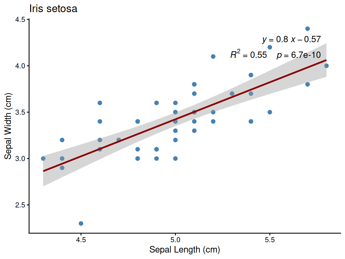
Example: Setosa species plot
6.6 File Organization
library(glue)

# Good practice: separate directory
fig_dir <- "figures"
dir.create(fig_dir, showWarnings = FALSE)

ggsave(glue("{fig_dir}/figure1.pdf"), p1, width = 7, height = 5)
ggsave(glue("{fig_dir}/figure1.png"), p1, width = 7, height = 5, dpi = 300)

# Save both vector and raster versions!
6.7 Using magick for Conversion
library(magick)

# Convert PDF to 300 DPI PNG
img <- image_read_pdf("plot.pdf", density = 300)
image_write(img, "plot.png", format = "png", quality = 100)

# With better antialiasing (remove alpha channel)
img <- image_read_pdf("plot.pdf", density = 300)
img <- image_background(img, "white")  # Remove alpha
image_write(img, "plot.png", format = "png", quality = 100)

# Batch convert all PDFs in directory
pdf_files <- list.files(pattern = "\\.pdf$")
for (file in pdf_files) {
  img <- image_read_pdf(file, density = 300)
  img <- image_background(img, "white")
  out_file <- sub("\\.pdf$", ".png", file)
  image_write(img, out_file, format = "png", quality = 100)
}
6.8 Batch Saving Multiple Plots
Make a plotting function
make_species_plot <- function(data, species) {
  ggplot(data, aes(x = Sepal.Length, y = Sepal.Width)) +
    geom_point(size = 2, color = "steelblue") +
    geom_smooth(method = "lm", se = TRUE, color = "darkred", formula = y ~ x) +
    labs(title = glue("Iris {species}"), x = "Sepal Length (cm)", y = "Sepal Width (cm)") +
    theme_classic(base_size = 12)
}
Nest data per Species
# Nest data by Species and apply plotting function
plot_data <- iris %>%
  nest(data = -Species) %>%
  mutate(plot = map2(data, Species, make_species_plot))
Write out to separate file per Species
# Save all plots using walk2
walk2(plot_data$plot, plot_data$Species, ~ggsave(
  filename = glue("{fig_dir}/iris_{..2}.pdf"),
  plot = ..1,
  width = 6, height = 5
))
# A tibble: 3 × 3
Species data plot
<fct> <list> <list>
1 setosa <tibble [50 × 4]> <ggplt2::>
2 versicolor <tibble [50 × 4]> <ggplt2::>
3 virginica <tibble [50 × 4]> <ggplt2::>head(plot_data$data[[1]])# A tibble: 6 × 4
Sepal.Length Sepal.Width Petal.Length Petal.Width
<dbl> <dbl> <dbl> <dbl>
1 5.1 3.5 1.4 0.2
2 4.9 3 1.4 0.2
3 4.7 3.2 1.3 0.2
4 4.6 3.1 1.5 0.2
5 5 3.6 1.4 0.2
6 5.4 3.9 1.7 0.4
plot_data$plot[[1]]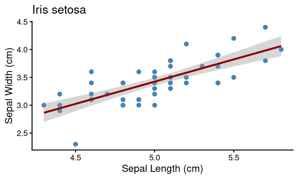
6.9 Recommendations
Best Practices
- Always use ggsave() for ggplot2 (not manual devices)
- Always specify width, height, units and DPI (for raster output)
- Increase DPI from the default for all raster formats set ≥300
- Use cairo_pdf for PDF output
- Save both PDF and PNG versions
- Organize figures in dedicated directory
6.10 Summary
Key Takeaways
Use
ggsave()for ggplot2 - never use manual devices or Export buttonAlways specify dimensions explicitly:
ggsave("plot.pdf", p, width = 7, height = 5, units = "in")Key parameters:
width,height,units- control sizedpi- resolution for raster (300+ for print)device- format override (e.g.,cairo_pdf)
Use
cairo_pdffor PDFs - better Unicode and font supportSave dual formats - PDF for publication, PNG for presentations/emails
Batch saving workflow:
- Create plotting function
- Use
walk()or loops to save multiple plots - Consistent naming scheme
Reproducibility - scripted saving ensures consistent output
Organize output - dedicated
figures/directory with meaningful names
6.11 Exercises
Try It Yourself
Create a plot and save it using
ggsave()with explicit parameters:p <- ggplot(mtcars, aes(mpg, hp)) + geom_point() ggsave("my_plot.pdf", p, width = 7, height = 5, device = cairo_pdf) ggsave("my_plot.png", p, width = 7, height = 5, dpi = 300)Create a function that saves both PDF and PNG:
save_dual <- function(filename, plot, ...) {
  ggsave(paste0(filename, ".pdf"), plot, device = cairo_pdf, ...)
  ggsave(paste0(filename, ".png"), plot, dpi = 300, ...)
}
Use
purrr::walk()to batch-save 5 different plotsCompare file sizes between 72 DPI and 300 DPI PNG
6.12 Further Reading
- ggsave() documentation - all parameters explained
- R Graphics Devices - comprehensive device reference
- Cairo graphics - font rendering library
- purrr iteration - functional programming for batch operations